Composing Programs

About

Online textbook of CS 61A: Structure and Interpretation of Computer Programs by Prof. John DeNero from University of California, Berkeley.

Preface

Welcome to Composing Programs, a free online introduction to programming and computer science.

In the tradition of SICP, this text focuses on methods for abstraction, programming paradigms, and techniques for managing the complexity of large programs. These concepts are illustrated primarily using the Python 3 programming language.

In addition to reading the chapters below, you can apply your knowledge to the programming projectsthat accompany the text and visualize program execution using the Online Python Tutor.

Instructors: If you are interested in adapting any of these materials for your courses, please fill out this short survey so that we can support your efforts.

Chapter 1: Building Abstractions with Functions

1.1 Getting Started

1.2 Elements of Programming

1.3 Defining New Functions

1.4 Designing Functions

1.5 Control

1.6 Higher-Order Functions

1.7 Recursive Functions

Chapter 2: Building Abstractions with Data

2.1 Introduction

2.2 Data Abstraction

2.3 Sequences

2.4 Mutable Data

2.5 Object-Oriented Programming

2.6 Implementing Classes and Objects

2.7 Object Abstraction

2.8 Efficiency

2.9 Recursive Objects

Chapter 3: Interpreting Computer Programs

3.1 Introduction

3.2 Functional Programming

3.3 Exceptions

3.4 Interpreters for Languages with Combination

3.5 Interpreters for Languages with Abstraction

Chapter 4: Data Processing

4.1 Introduction

4.2 Implicit Sequences

4.3 Declarative Programming

4.4 Logic Programming

4.5 Unification

4.6 Distributed Computing

4.7 Distributed Data Processing

4.8 Parallel Computing

Chapter 1: Building Abstractions with Functions

1.1 Getting Started

Computer science is a tremendously broad academic discipline. The areas of globally distributed systems, artificial intelligence, robotics, graphics, security, scientific computing, computer architecture, and dozens of emerging sub-fields all expand with new techniques and discoveries every year. The rapid progress of computer science has left few aspects of human life unaffected. Commerce, communication, science, art, leisure, and politics have all been reinvented as computational domains.

The high productivity of computer science is only possible because the discipline is built upon an elegant and powerful set of fundamental ideas. All computing begins with representing information, specifying logic to process it, and designing abstractions that manage the complexity of that logic. Mastering these fundamentals will require us to understand precisely how computers interpret computer programs and carry out computational processes.

These fundamental ideas have long been taught using the classic textbook Structure and Interpretation of Computer Programs (SICP) by Harold Abelson and Gerald Jay Sussman with Julie Sussman. This text borrows heavily from that textbook, which the original authors have kindly licensed for adaptation and reuse under a Creative Commons license. These notes are published under the Creative Commons attribution non-commericial share-alike license version 3.

1.1.1 Programming in Python

A language isn’t something you learn so much as something you join.

—Arika Okrent

In order to define computational processes, we need a programming language; preferably one that many humans and a great variety of computers can all understand. In this text, we will work primarily with the Python language.

Python is a widely used programming language that has recruited enthusiasts from many professions: web programmers, game engineers, scientists, academics, and even designers of new programming languages. When you learn Python, you join a million-person-strong community of developers. Developer communities are tremendously important institutions: members help each other solve problems, share their projects and experiences, and collectively develop software and tools. Dedicated members often achieve celebrity and widespread esteem for their contributions.

The Python language itself is the product of a large volunteer community that prides itself on the diversityof its contributors. The language was conceived and first implemented by Guido van Rossum in the late 1980’s. The first chapter of his Python 3 Tutorial explains why Python is so popular, among the many languages available today.

Python excels as an instructional language because, throughout its history, Python’s developers have emphasized the human interpretability of Python code, reinforced by the Zen of Python guiding principles of beauty, simplicity, and readability. Python is particularly appropriate for this text because its broad set of features support a variety of different programming styles, which we will explore. While there is no single way to program in Python, there are a set of conventions shared across the developer community that facilitate reading, understanding, and extending existing programs. Python’s combination of great flexibility and accessibility allows students to explore many programming paradigms, and then apply their newly acquired knowledge to thousands of ongoing projects.

These notes maintain the spirit of SICP by introducing the features of Python in step with techniques for abstraction and a rigorous model of computation. In addition, these notes provide a practical introduction to Python programming, including some advanced language features and illustrative examples. Increasing your facility with Python should come naturally as you progress through the text.

The best way to get started programming in Python is to interact with the interpreter directly. This section describes how to install Python 3, initiate an interactive session with the interpreter, and start programming.

1.1.2 Installing Python 3

As with all great software, Python has many versions. This text will use the most recent stable version of Python 3. Many computers have older versions of Python installed already, such as Python 2.7, but those will not match the descriptions in this text. You should be able to use any computer, but expect to install Python 3. (Don’t worry, Python is free.)

You can download Python 3 from the Python downloads page by clicking on the version that begins with 3 (not 2). Follow the instructions of the installer to complete installation.

For further guidance, try these video tutorials on Windows installation and Mac installation of Python 3, created by Julia Oh.

1.1.3 Interactive Sessions

In an interactive Python session, you type some Python code after the prompt, >>>. The Python interpreter reads and executes what you type, carrying out your various commands.

To start an interactive session, run the Python 3 application. Type python3 at a terminal prompt (Mac/Unix/Linux) or open the Python 3 application in Windows.

If you see the Python prompt, >>>, then you have successfully started an interactive session. These notes depict example interactions using the prompt, followed by some input.

>>> 2 + 2
4

Interactive controls. Each session keeps a history of what you have typed. To access that history, press -P (previous) and -N (next). -D exits a session, which discards this history. Up and down arrows also cycle through history on some systems.

1.1.4 First Example

And, as imagination bodies forth

The forms of things to unknown, and the poet’s pen

Turns them to shapes, and gives to airy nothing

A local habitation and a name.

—William Shakespeare, A Midsummer-Night’s Dream

To give Python a proper introduction, we will begin with an example that uses several language features. In the next section, we will start from scratch and build up the language piece by piece. Think of this section as a sneak preview of features to come.

Python has built-in support for a wide range of common programming activities, such as manipulating text, displaying graphics, and communicating over the Internet. The line of Python code

>>> from urllib.request import urlopen

is an import statement that loads functionality for accessing data on the Internet. In particular, it makes available a function called urlopen, which can access the content at a uniform resource locator (URL), a location of something on the Internet.

Statements & Expressions. Python code consists of expressions and statements. Broadly, computer programs consist of instructions to either

1. Compute some value
2. Carry out some action

Statements typically describe actions. When the Python interpreter executes a statement, it carries out the corresponding action. On the other hand, expressions typically describe computations. When Python evaluates an expression, it computes the value of that expression. This chapter introduces several types of statements and expressions.

The assignment statement

>>> shakespeare = urlopen('http://composingprograms.com/shakespeare.txt')

associates the name shakespeare with the value of the expression that follows =. That expression applies the urlopen function to a URL that contains the complete text of William Shakespeare’s 37 plays, all in a single text document.

Functions. Functions encapsulate logic that manipulates data. urlopen is a function. A web address is a piece of data, and the text of Shakespeare’s plays is another. The process by which the former leads to the latter may be complex, but we can apply that process using only a simple expression because that complexity is tucked away within a function. Functions are the primary topic of this chapter.

Another assignment statement

>>> words = set(shakespeare.read().decode().split())

associates the name words to the set of all unique words that appear in Shakespeare’s plays, all 33,721 of them. The chain of commands to read, decode, and split, each operate on an intermediate computational entity: we read the data from the opened URL, then decode the data into text, and finally split the text into words. All of those words are placed in a set.

Objects. A set is a type of object, one that supports set operations like computing intersections and membership. An object seamlessly bundles together data and the logic that manipulates that data, in a way that manages the complexity of both. Objects are the primary topic of Chapter 2. Finally, the expression

>>> {w for w in words if len(w) == 6 and w[::-1] in words}
{'redder', 'drawer', 'reward', 'diaper', 'repaid'}

is a compound expression that evaluates to the set of all Shakespearian words that are simultaneously a word spelled in reverse. The cryptic notation w[::-1] enumerates each letter in a word, but the -1dictates to step backwards. When you enter an expression in an interactive session, Python prints its value on the following line.

Interpreters. Evaluating compound expressions requires a precise procedure that interprets code in a predictable way. A program that implements such a procedure, evaluating compound expressions, is called an interpreter. The design and implementation of interpreters is the primary topic of Chapter 3.

When compared with other computer programs, interpreters for programming languages are unique in their generality. Python was not designed with Shakespeare in mind. However, its great flexibility allowed us to process a large amount of text with only a few statements and expressions.

In the end, we will find that all of these core concepts are closely related: functions are objects, objects are functions, and interpreters are instances of both. However, developing a clear understanding of each of these concepts and their role in organizing code is critical to mastering the art of programming.

1.1.5 Errors

Python is waiting for your command. You are encouraged to experiment with the language, even though you may not yet know its full vocabulary and structure. However, be prepared for errors. While computers are tremendously fast and flexible, they are also extremely rigid. The nature of computers is described in Stanford’s introductory course as

The fundamental equation of computers is:

computer = powerful + stupid

Computers are very powerful, looking at volumes of data very quickly. Computers can perform billions of operations per second, where each operation is pretty simple.

Computers are also shockingly stupid and fragile. The operations that they can do are extremely rigid, simple, and mechanical. The computer lacks anything like real insight … it’s nothing like the HAL 9000 from the movies. If nothing else, you should not be intimidated by the computer as if it’s some sort of brain. It’s very mechanical underneath it all.

Programming is about a person using their real insight to build something useful, constructed out of these teeny, simple little operations that the computer can do.

—Francisco Cai and Nick Parlante, Stanford CS101

The rigidity of computers will immediately become apparent as you experiment with the Python interpreter: even the smallest spelling and formatting changes will cause unexpected output and errors.

Learning to interpret errors and diagnose the cause of unexpected errors is called debugging. Some guiding principles of debugging are:

1. Test incrementally: Every well-written program is composed of small, modular components that can be tested individually. Try out everything you write as soon as possible to identify problems early and gain confidence in your components.
2. Isolate errors: An error in the output of a statement can typically be attributed to a particular modular component. When trying to diagnose a problem, trace the error to the smallest fragment of code you can before trying to correct it.
3. Check your assumptions: Interpreters do carry out your instructions to the letter — no more and no less. Their output is unexpected when the behavior of some code does not match what the programmer believes (or assumes) that behavior to be. Know your assumptions, then focus your debugging effort on verifying that your assumptions actually hold.
4. Consult others: You are not alone! If you don’t understand an error message, ask a friend, instructor, or search engine. If you have isolated an error, but can’t figure out how to correct it, ask someone else to take a look. A lot of valuable programming knowledge is shared in the process of group problem solving.

Incremental testing, modular design, precise assumptions, and teamwork are themes that persist throughout this text. Hopefully, they will also persist throughout your computer science career.

1.2 Elements of Programming

A programming language is more than just a means for instructing a computer to perform tasks. The language also serves as a framework within which we organize our ideas about computational processes. Programs serve to communicate those ideas among the members of a programming community. Thus, programs must be written for people to read, and only incidentally for machines to execute.

When we describe a language, we should pay particular attention to the means that the language provides for combining simple ideas to form more complex ideas. Every powerful language has three such mechanisms:

• primitive expressions and statements, which represent the simplest building blocks that the language provides,
• means of combination, by which compound elements are built from simpler ones, and
• means of abstraction, by which compound elements can be named and manipulated as units.

In programming, we deal with two kinds of elements: functions and data. (Soon we will discover that they are really not so distinct.) Informally, data is stuff that we want to manipulate, and functions describe the rules for manipulating the data. Thus, any powerful programming language should be able to describe primitive data and primitive functions, as well as have some methods for combining and abstracting both functions and data.

1.2.1 Expressions

Video: Show Hide

Having experimented with the full Python interpreter in the previous section, we now start anew, methodically developing the Python language element by element. Be patient if the examples seem simplistic — more exciting material is soon to come.

We begin with primitive expressions. One kind of primitive expression is a number. More precisely, the expression that you type consists of the numerals that represent the number in base 10.

>>> 42
42

Expressions representing numbers may be combined with mathematical operators to form a compound expression, which the interpreter will evaluate:

>>> -1 - -1
0
>>> 1/2 + 1/4 + 1/8 + 1/16 + 1/32 + 1/64 + 1/128
0.9921875

These mathematical expressions use infix notation, where the operator (e.g., +, -, *, or /) appears in between the operands (numbers). Python includes many ways to form compound expressions. Rather than attempt to enumerate them all immediately, we will introduce new expression forms as we go, along with the language features that they support.

1.2.2 Call Expressions

Video: Show Hide

The most important kind of compound expression is a call expression, which applies a function to some arguments. Recall from algebra that the mathematical notion of a function is a mapping from some input arguments to an output value. For instance, the max function maps its inputs to a single output, which is the largest of the inputs. The way in which Python expresses function application is the same as in conventional mathematics.

>>> max(7.5, 9.5)
9.5

This call expression has subexpressions: the operator is an expression that precedes parentheses, which enclose a comma-delimited list of operand expressions.

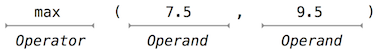
The operator specifies a function. When this call expression is evaluated, we say that the function max is called with arguments 7.5 and 9.5, and returns a value of 9.5.

The order of the arguments in a call expression matters. For instance, the function pow raises its first argument to the power of its second argument.

>>> pow(100, 2)
10000
>>> pow(2, 100)
1267650600228229401496703205376

Function notation has three principal advantages over the mathematical convention of infix notation. First, functions may take an arbitrary number of arguments:

>>> max(1, -2, 3, -4)
3

No ambiguity can arise, because the function name always precedes its arguments.

Second, function notation extends in a straightforward way to nested expressions, where the elements are themselves compound expressions. In nested call expressions, unlike compound infix expressions, the structure of the nesting is entirely explicit in the parentheses.

>>> max(min(1, -2), min(pow(3, 5), -4))
-2

There is no limit (in principle) to the depth of such nesting and to the overall complexity of the expressions that the Python interpreter can evaluate. However, humans quickly get confused by multi-level nesting. An important role for you as a programmer is to structure expressions so that they remain interpretable by yourself, your programming partners, and other people who may read your expressions in the future.

Third, mathematical notation has a great variety of forms: multiplication appears between terms, exponents appear as superscripts, division as a horizontal bar, and a square root as a roof with slanted siding. Some of this notation is very hard to type! However, all of this complexity can be unified via the notation of call expressions. While Python supports common mathematical operators using infix notation (like + and -), any operator can be expressed as a function with a name.

1.2.3 Importing Library Functions

Python defines a very large number of functions, including the operator functions mentioned in the preceding section, but does not make all of their names available by default. Instead, it organizes the functions and other quantities that it knows about into modules, which together comprise the Python Library. To use these elements, one imports them. For example, the math module provides a variety of familiar mathematical functions:

>>> from math import sqrt
>>> sqrt(256)
16.0

and the operator module provides access to functions corresponding to infix operators:

>>> from operator import add, sub, mul
>>> add(14, 28)
42
>>> sub(100, mul(7, add(8, 4)))
16

An import statement designates a module name (e.g., operator or math), and then lists the named attributes of that module to import (e.g., sqrt). Once a function is imported, it can be called multiple times.

There is no difference between using these operator functions (e.g., add) and the operator symbols themselves (e.g., +). Conventionally, most programmers use symbols and infix notation to express simple arithmetic.

The Python 3 Library Docs list the functions defined by each module, such as the math module. However, this documentation is written for developers who know the whole language well. For now, you may find that experimenting with a function tells you more about its behavior than reading the documentation. As you become familiar with the Python language and vocabulary, this documentation will become a valuable reference source.

1.2.4 Names and the Environment

Video: Show Hide

A critical aspect of a programming language is the means it provides for using names to refer to computational objects. If a value has been given a name, we say that the name binds to the value.

In Python, we can establish new bindings using the assignment statement, which contains a name to the left of = and a value to the right:

>>> radius = 10
>>> radius
10
>>> 2 * radius
20

Names are also bound via import statements.

>>> from math import pi
>>> pi * 71 / 223
1.0002380197528042

The = symbol is called the assignment operator in Python (and many other languages). Assignment is our simplest means of abstraction, for it allows us to use simple names to refer to the results of compound operations, such as the area computed above. In this way, complex programs are constructed by building, step by step, computational objects of increasing complexity.

The possibility of binding names to values and later retrieving those values by name means that the interpreter must maintain some sort of memory that keeps track of the names, values, and bindings. This memory is called an environment.

Names can also be bound to functions. For instance, the name max is bound to the max function we have been using. Functions, unlike numbers, are tricky to render as text, so Python prints an identifying description instead, when asked to describe a function:

>>> max
<built-in function max>

We can use assignment statements to give new names to existing functions.

>>> f = max
>>> f
<built-in function max>
>>> f(2, 3, 4)
4

And successive assignment statements can rebind a name to a new value.

>>> f = 2
>>> f
2

In Python, names are often called variable names or variables because they can be bound to different values in the course of executing a program. When a name is bound to a new value through assignment, it is no longer bound to any previous value. One can even bind built-in names to new values.

>>> max = 5
>>> max
5

After assigning max to 5, the name max is no longer bound to a function, and so attempting to call max(2, 3, 4) will cause an error.

When executing an assignment statement, Python evaluates the expression to the right of = before changing the binding to the name on the left. Therefore, one can refer to a name in right-side expression, even if it is the name to be bound by the assignment statement.

>>> x = 2
>>> x = x + 1
>>> x
3

We can also assign multiple values to multiple names in a single statement, where names on the left of =and expressions on the right of = are separated by commas.

>>> area, circumference = pi * radius * radius, 2 * pi * radius
>>> area
314.1592653589793
>>> circumference
62.83185307179586

Changing the value of one name does not affect other names. Below, even though the name area was bound to a value defined originally in terms of radius, the value of area has not changed. Updating the value of area requires another assignment statement.

>>> radius = 11
>>> area
314.1592653589793
>>> area = pi * radius * radius
380.132711084365

With multiple assignment, all expressions to the right of = are evaluated before any names to the left are bound to those values. As a result of this rule, swapping the values bound to two names can be performed in a single statement.

>>> x, y = 3, 4.5
>>> y, x = x, y
>>> x
4.5
>>> y
3

1.2.5 Evaluating Nested Expressions

One of our goals in this chapter is to isolate issues about thinking procedurally. As a case in point, let us consider that, in evaluating nested call expressions, the interpreter is itself following a procedure.

To evaluate a call expression, Python will do the following:

1. Evaluate the operator and operand subexpressions, then
2. Apply the function that is the value of the operator subexpression to the arguments that are the values of the operand subexpressions.

Even this simple procedure illustrates some important points about processes in general. The first step dictates that in order to accomplish the evaluation process for a call expression we must first evaluate other expressions. Thus, the evaluation procedure is recursive in nature; that is, it includes, as one of its steps, the need to invoke the rule itself.

For example, evaluating

>>> sub(pow(2, add(1, 10)), pow(2, 5))
2016

requires that this evaluation procedure be applied four times. If we draw each expression that we evaluate, we can visualize the hierarchical structure of this process.

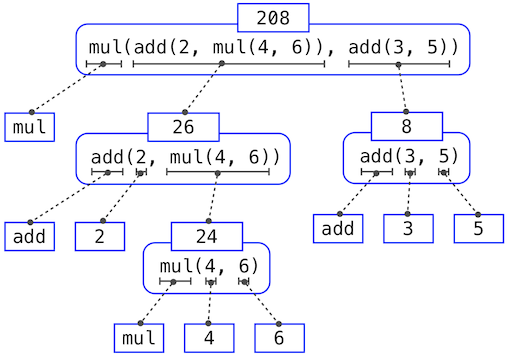
This illustration is called an expression tree. In computer science, trees conventionally grow from the top down. The objects at each point in a tree are called nodes; in this case, they are expressions paired with their values.

Evaluating its root, the full expression at the top, requires first evaluating the branches that are its subexpressions. The leaf expressions (that is, nodes with no branches stemming from them) represent either functions or numbers. The interior nodes have two parts: the call expression to which our evaluation rule is applied, and the result of that expression. Viewing evaluation in terms of this tree, we can imagine that the values of the operands percolate upward, starting from the terminal nodes and then combining at higher and higher levels.

Next, observe that the repeated application of the first step brings us to the point where we need to evaluate, not call expressions, but primitive expressions such as numerals (e.g., 2) and names (e.g., add). We take care of the primitive cases by stipulating that

• A numeral evaluates to the number it names,
• A name evaluates to the value associated with that name in the current environment.

Notice the important role of an environment in determining the meaning of the symbols in expressions. In Python, it is meaningless to speak of the value of an expression such as

>>> add(x, 1)

without specifying any information about the environment that would provide a meaning for the name x(or even for the name add). Environments provide the context in which evaluation takes place, which plays an important role in our understanding of program execution.

This evaluation procedure does not suffice to evaluate all Python code, only call expressions, numerals, and names. For instance, it does not handle assignment statements. Executing

>>> x = 3

does not return a value nor evaluate a function on some arguments, since the purpose of assignment is instead to bind a name to a value. In general, statements are not evaluated but executed; they do not produce a value but instead make some change. Each type of expression or statement has its own evaluation or execution procedure.

A pedantic note: when we say that “a numeral evaluates to a number,” we actually mean that the Python interpreter evaluates a numeral to a number. It is the interpreter which endows meaning to the programming language. Given that the interpreter is a fixed program that always behaves consistently, we can say that numerals (and expressions) themselves evaluate to values in the context of Python programs.

1.2.6 The Non-Pure Print Function

Video: Show Hide

Throughout this text, we will distinguish between two types of functions.

Pure functions. Functions have some input (their arguments) and return some output (the result of applying them). The built-in function

>>> abs(-2)
2

can be depicted as a small machine that takes input and produces output.

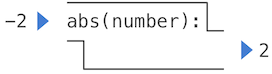
The function abs is pure. Pure functions have the property that applying them has no effects beyond returning a value. Moreover, a pure function must always return the same value when called twice with the same arguments.

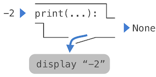
Non-pure functions. In addition to returning a value, applying a non-pure function can generate side effects, which make some change to the state of the interpreter or computer. A common side effect is to generate additional output beyond the return value, using the print function.

>>> print(1, 2, 3)
1 2 3

While print and abs may appear to be similar in these examples, they work in fundamentally different ways. The value that print returns is always None, a special Python value that represents nothing. The interactive Python interpreter does not automatically print the value None. In the case of print, the function itself is printing output as a side effect of being called.

A nested expression of calls to print highlights the non-pure character of the function.

>>> print(print(1), print(2))
1
2
None None

If you find this output to be unexpected, draw an expression tree to clarify why evaluating this expression produces this peculiar output.

Be careful with print! The fact that it returns None means that it should not be the expression in an assignment statement.

>>> two = print(2)
2
>>> print(two)
None

Pure functions are restricted in that they cannot have side effects or change behavior over time. Imposing these restrictions yields substantial benefits. First, pure functions can be composed more reliably into compound call expressions. We can see in the non-pure function example above that printdoes not return a useful result when used in an operand expression. On the other hand, we have seen that functions such as max, pow and sqrt can be used effectively in nested expressions.

Second, pure functions tend to be simpler to test. A list of arguments will always lead to the same return value, which can be compared to the expected return value. Testing is discussed in more detail later in this chapter.

Third, Chapter 4 will illustrate that pure functions are essential for writing concurrent programs, in which multiple call expressions may be evaluated simultaneously.

By contrast, Chapter 2 investigates a range of non-pure functions and describes their uses.

For these reasons, we concentrate heavily on creating and using pure functions in the remainder of this chapter. The print function is only used so that we can see the intermediate results of computations.

1.3 Defining New Functions

Video: Show Hide

We have identified in Python some of the elements that must appear in any powerful programming language:

1. Numbers and arithmetic operations are primitive built-in data values and functions.
2. Nested function application provides a means of combining operations.
3. Binding names to values provides a limited means of abstraction.

Now we will learn about function definitions, a much more powerful abstraction technique by which a name can be bound to compound operation, which can then be referred to as a unit.

We begin by examining how to express the idea of squaring. We might say, “To square something, multiply it by itself.” This is expressed in Python as

>>> def square(x):
        return mul(x, x)

which defines a new function that has been given the name square. This user-defined function is not built into the interpreter. It represents the compound operation of multiplying something by itself. The x in this definition is called a formal parameter, which provides a name for the thing to be multiplied. The definition creates this user-defined function and associates it with the name square.

How to define a function. Function definitions consist of a def statement that indicates a and a comma-separated list of named, then a return statement, called the function body, that specifies the `` of the function, which is an expression to be evaluated whenever the function is applied:

def <name>(<formal parameters>):
    return <return expression>

The second line must be indented — most programmers use four spaces to indent. The return expression is not evaluated right away; it is stored as part of the newly defined function and evaluated only when the function is eventually applied.

Having defined square, we can apply it with a call expression:

>>> square(21)
441
>>> square(add(2, 5))
49
>>> square(square(3))
81

We can also use square as a building block in defining other functions. For example, we can easily define a function sum_squares that, given any two numbers as arguments, returns the sum of their squares:

>>> def sum_squares(x, y):
        return add(square(x), square(y))
>>> sum_squares(3, 4)
25

User-defined functions are used in exactly the same way as built-in functions. Indeed, one cannot tell from the definition of sum_squares whether square is built into the interpreter, imported from a module, or defined by the user.

Both def statements and assignment statements bind names to values, and any existing bindings are lost. For example, g below first refers to a function of no arguments, then a number, and then a different function of two arguments.

>>> def g():
        return 1
>>> g()
1
>>> g = 2
>>> g
2
>>> def g(h, i):
        return h + i
>>> g(1, 2)
3

1.3.1 Environments

Video: Show Hide

Our subset of Python is now complex enough that the meaning of programs is non-obvious. What if a formal parameter has the same name as a built-in function? Can two functions share names without confusion? To resolve such questions, we must describe environments in more detail.

An environment in which an expression is evaluated consists of a sequence of frames, depicted as boxes. Each frame contains bindings, each of which associates a name with its corresponding value. There is a single global frame. Assignment and import statements add entries to the first frame of the current environment. So far, our environment consists only of the global frame.

from math import pi
tau = 2 * pi

This environment diagram shows the bindings of the current environment, along with the values to which names are bound. The environment diagrams in this text are interactive: you can step through the lines of the small program on the left to see the state of the environment evolve on the right. You can also click on the “Edit code in Online Python Tutor” link to load the example into the Online Python Tutor, a tool created by Philip Guo for generating these environment diagrams. You are encouraged to create examples yourself and study the resulting environment diagrams.

Functions appear in environment diagrams as well. An import statement binds a name to a built-in function. A def statement binds a name to a user-defined function created by the definition. The resulting environment after importing mul and defining square appears below:

from operator import mul
def square(x):
    return mul(x, x)

Each function is a line that starts with func, followed by the function name and formal parameters. Built-in functions such as mul do not have formal parameter names, and so ... is always used instead.

The name of a function is repeated twice, once in the frame and again as part of the function itself. The name appearing in the function is called the intrinsic name. The name in a frame is a bound name. There is a difference between the two: different names may refer to the same function, but that function itself has only one intrinsic name.

The name bound to a function in a frame is the one used during evaluation. The intrinsic name of a function does not play a role in evaluation. Step through the example below using the Forward button to see that once the name max is bound to the value 3, it can no longer be used as a function.

f = max
max = 3
result = f(2, 3, 4)
max(1, 2)  # Causes an error

The error message TypeError: 'int' object is not callable is reporting that the name max (currently bound to the number 3) is an integer and not a function. Therefore, it cannot be used as the operator in a call expression.

Function Signatures. Functions differ in the number of arguments that they are allowed to take. To track these requirements, we draw each function in a way that shows the function name and its formal parameters. The user-defined function square takes only x; providing more or fewer arguments will result in an error. A description of the formal parameters of a function is called the function’s signature.

The function max can take an arbitrary number of arguments. It is rendered as max(...). Regardless of the number of arguments taken, all built-in functions will be rendered as (...), because these primitive functions were never explicitly defined.

1.3.2 Calling User-Defined Functions

To evaluate a call expression whose operator names a user-defined function, the Python interpreter follows a computational process. As with any call expression, the interpreter evaluates the operator and operand expressions, and then applies the named function to the resulting arguments.

Applying a user-defined function introduces a second local frame, which is only accessible to that function. To apply a user-defined function to some arguments:

1. Bind the arguments to the names of the function’s formal parameters in a new local frame.
2. Execute the body of the function in the environment that starts with this frame.

The environment in which the body is evaluated consists of two frames: first the local frame that contains formal parameter bindings, then the global frame that contains everything else. Each instance of a function application has its own independent local frame.

To illustrate an example in detail, several steps of the environment diagram for the same example are depicted below. After executing the first import statement, only the name mul is bound in the global frame.

from operator import mul
def square(x):
    return mul(x, x)
square(-2)

First, the definition statement for the function square is executed. Notice that the entire def statement is processed in a single step. The body of a function is not executed until the function is called (not when it is defined).

Next, The square function is called with the argument -2, and so a new frame is created with the formal parameter x bound to the value -2.

Then, the name x is looked up in the current environment, which consists of the two frames shown. In both occurrences, x evaluates to -2, and so the square function returns 4.

The “Return value” in the square() frame is not a name binding; instead it indicates the value returned by the function call that created the frame.

Even in this simple example, two different environments are used. The top-level expression square(-2) is evaluated in the global environment, while the return expression mul(x, x) is evaluated in the environment created for by calling square. Both x and mul are bound in this environment, but in different frames.

The order of frames in an environment affects the value returned by looking up a name in an expression. We stated previously that a name is evaluated to the value associated with that name in the current environment. We can now be more precise:

Name Evaluation. A name evaluates to the value bound to that name in the earliest frame of the current environment in which that name is found.

Our conceptual framework of environments, names, and functions constitutes a model of evaluation; while some mechanical details are still unspecified (e.g., how a binding is implemented), our model does precisely and correctly describe how the interpreter evaluates call expressions. In Chapter 3 we will see how this model can serve as a blueprint for implementing a working interpreter for a programming language.

1.3.3 Example: Calling a User-Defined Function

Let us again consider our two simple function definitions and illustrate the process that evaluates a call expression for a user-defined function.

from operator import add, mul
def square(x):
    return mul(x, x)

def sum_squares(x, y):
    return add(square(x), square(y))

result = sum_squares(5, 12)

Python first evaluates the name sum_squares, which is bound to a user-defined function in the global frame. The primitive numeric expressions 5 and 12 evaluate to the numbers they represent.

Next, Python applies sum_squares, which introduces a local frame that binds x to 5 and y to 12.

The body of sum_squares contains this call expression:

  add     (  square(x)  ,  square(y)  )
________     _________     _________
operator     operand 0     operand 1

All three subexpressions are evaluated in the current environment, which begins with the frame labeled sum_squares(). The operator subexpression add is a name found in the global frame, bound to the built-in function for addition. The two operand subexpressions must be evaluated in turn, before addition is applied. Both operands are evaluated in the current environment beginning with the frame labeled sum_squares.

In operand 0, square names a user-defined function in the global frame, while x names the number 5 in the local frame. Python applies square to 5 by introducing yet another local frame that binds x to 5.

Using this environment, the expression mul(x, x) evaluates to 25.

Our evaluation procedure now turns to operand 1, for which y names the number 12. Python evaluates the body of square again, this time introducing yet another local frame that binds x to 12. Hence, operand 1 evaluates to 144.

Finally, applying addition to the arguments 25 and 144 yields a final return value for sum_squares: 169.

This example illustrates many of the fundamental ideas we have developed so far. Names are bound to values, which are distributed across many independent local frames, along with a single global frame that contains shared names. A new local frame is introduced every time a function is called, even if the same function is called twice.

All of this machinery exists to ensure that names resolve to the correct values at the correct times during program execution. This example illustrates why our model requires the complexity that we have introduced. All three local frames contain a binding for the name x, but that name is bound to different values in different frames. Local frames keep these names separate.

1.3.4 Local Names

One detail of a function’s implementation that should not affect the function’s behavior is the implementer’s choice of names for the function’s formal parameters. Thus, the following functions should provide the same behavior:

>>> def square(x):
        return mul(x, x)
>>> def square(y):
        return mul(y, y)

This principle — that the meaning of a function should be independent of the parameter names chosen by its author — has important consequences for programming languages. The simplest consequence is that the parameter names of a function must remain local to the body of the function.

If the parameters were not local to the bodies of their respective functions, then the parameter x in square could be confused with the parameter x in sum_squares. Critically, this is not the case: the binding for x in different local frames are unrelated. The model of computation is carefully designed to ensure this independence.

We say that the scope of a local name is limited to the body of the user-defined function that defines it. When a name is no longer accessible, it is out of scope. This scoping behavior isn’t a new fact about our model; it is a consequence of the way environments work.

1.3.5 Choosing Names

The interchangeability of names does not imply that formal parameter names do not matter at all. On the contrary, well-chosen function and parameter names are essential for the human interpretability of function definitions!

The following guidelines are adapted from the style guide for Python code, which serves as a guide for all (non-rebellious) Python programmers. A shared set of conventions smooths communication among members of a developer community. As a side effect of following these conventions, you will find that your code becomes more internally consistent.

1. Function names are lowercase, with words separated by underscores. Descriptive names are encouraged.
2. Function names typically evoke operations applied to arguments by the interpreter (e.g., print, add, square) or the name of the quantity that results (e.g., max, abs, sum).
3. Parameter names are lowercase, with words separated by underscores. Single-word names are preferred.
4. Parameter names should evoke the role of the parameter in the function, not just the kind of argument that is allowed.
5. Single letter parameter names are acceptable when their role is obvious, but avoid “l” (lowercase ell), “O” (capital oh), or “I” (capital i) to avoid confusion with numerals.

There are many exceptions to these guidelines, even in the Python standard library. Like the vocabulary of the English language, Python has inherited words from a variety of contributors, and the result is not always consistent.

1.3.6 Functions as Abstractions

Though it is very simple, sum_squares exemplifies the most powerful property of user-defined functions. The function sum_squares is defined in terms of the function square, but relies only on the relationship that square defines between its input arguments and its output values.

We can write sum_squares without concerning ourselves with how to square a number. The details of how the square is computed can be suppressed, to be considered at a later time. Indeed, as far as sum_squares is concerned, square is not a particular function body, but rather an abstraction of a function, a so-called functional abstraction. At this level of abstraction, any function that computes the square is equally good.

Thus, considering only the values they return, the following two functions for squaring a number should be indistinguishable. Each takes a numerical argument and produces the square of that number as the value.

>>> def square(x):
        return mul(x, x)
>>> def square(x):
        return mul(x, x-1) + x

In other words, a function definition should be able to suppress details. The users of the function may not have written the function themselves, but may have obtained it from another programmer as a “black box”. A programmer should not need to know how the function is implemented in order to use it. The Python Library has this property. Many developers use the functions defined there, but few ever inspect their implementation.

Aspects of a functional abstraction. To master the use of a functional abstraction, it is often useful to consider its three core attributes. The domain of a function is the set of arguments it can take. The rangeof a function is the set of values it can return. The intent of a function is the relationship it computes between inputs and output (as well as any side effects it might generate). Understanding functional abstractions via their domain, range, and intent is critical to using them correctly in a complex program.

For example, any square function that we use to implement sum_squares should have these attributes:

• The domain is any single real number.
• The range is any non-negative real number.
• The intent is that the output is the square of the input.

These attributes do not specify how the intent is carried out; that detail is abstracted away.

1.3.7 Operators

Video: Show Hide

Mathematical operators (such as + and -) provided our first example of a method of combination, but we have yet to define an evaluation procedure for expressions that contain these operators.

Python expressions with infix operators each have their own evaluation procedures, but you can often think of them as short-hand for call expressions. When you see

>>> 2 + 3
5

simply consider it to be short-hand for

>>> add(2, 3)
5

Infix notation can be nested, just like call expressions. Python applies the normal mathematical rules of operator precedence, which dictate how to interpret a compound expression with multiple operators.

>>> 2 + 3 * 4 + 5
19

evaluates to the same result as

>>> add(add(2, mul(3, 4)), 5)
19

The nesting in the call expression is more explicit than the operator version, but also harder to read. Python also allows subexpression grouping with parentheses, to override the normal precedence rules or make the nested structure of an expression more explicit.

>>> (2 + 3) * (4 + 5)
45

evaluates to the same result as

>>> mul(add(2, 3), add(4, 5))
45

When it comes to division, Python provides two infix operators: / and //. The former is normal division, so that it results in a floating point, or decimal value, even if the divisor evenly divides the dividend:

>>> 5 / 4
1.25
>>> 8 / 4
2.0

The // operator, on the other hand, rounds the result down to an integer:

>>> 5 // 4
1
>>> -5 // 4
-2

These two operators are shorthand for the truediv and floordiv functions.

>>> from operator import truediv, floordiv
>>> truediv(5, 4)
1.25
>>> floordiv(5, 4)
1

You should feel free to use infix operators and parentheses in your programs. Idiomatic Python prefers operators over call expressions for simple mathematical operations.

1.4 Designing Functions

Video: Show Hide

Functions are an essential ingredient of all programs, large and small, and serve as our primary medium to express computational processes in a programming language. So far, we have discussed the formal properties of functions and how they are applied. We now turn to the topic of what makes a good function. Fundamentally, the qualities of good functions all reinforce the idea that functions are abstractions.

• Each function should have exactly one job. That job should be identifiable with a short name and characterizable in a single line of text. Functions that perform multiple jobs in sequence should be divided into multiple functions.
• Don’t repeat yourself is a central tenet of software engineering. The so-called DRY principle states that multiple fragments of code should not describe redundant logic. Instead, that logic should be implemented once, given a name, and applied multiple times. If you find yourself copying and pasting a block of code, you have probably found an opportunity for functional abstraction.
• Functions should be defined generally. Squaring is not in the Python Library precisely because it is a special case of the pow function, which raises numbers to arbitrary powers.

These guidelines improve the readability of code, reduce the number of errors, and often minimize the total amount of code written. Decomposing a complex task into concise functions is a skill that takes experience to master. Fortunately, Python provides several features to support your efforts.

1.4.1 Documentation

A function definition will often include documentation describing the function, called a docstring, which must be indented along with the function body. Docstrings are conventionally triple quoted. The first line describes the job of the function in one line. The following lines can describe arguments and clarify the behavior of the function:

>>> def pressure(v, t, n):
        """Compute the pressure in pascals of an ideal gas.

        Applies the ideal gas law: http://en.wikipedia.org/wiki/Ideal_gas_law

        v -- volume of gas, in cubic meters
        t -- absolute temperature in degrees kelvin
        n -- particles of gas
        """
        k = 1.38e-23  # Boltzmann's constant
        return n * k * t / v

When you call help with the name of a function as an argument, you see its docstring (type q to quit Python help).

>>> help(pressure)

When writing Python programs, include docstrings for all but the simplest functions. Remember, code is written only once, but often read many times. The Python docs include docstring guidelines that maintain consistency across different Python projects.

Comments. Comments in Python can be attached to the end of a line following the # symbol. For example, the comment Boltzmann's constant above describes k. These comments don’t ever appear in Python’s help, and they are ignored by the interpreter. They exist for humans alone.

1.4.2 Default Argument Values

A consequence of defining general functions is the introduction of additional arguments. Functions with many arguments can be awkward to call and difficult to read.

In Python, we can provide default values for the arguments of a function. When calling that function, arguments with default values are optional. If they are not provided, then the default value is bound to the formal parameter name instead. For instance, if an application commonly computes pressure for one mole of particles, this value can be provided as a default:

>>> def pressure(v, t, n=6.022e23):
        """Compute the pressure in pascals of an ideal gas.

        v -- volume of gas, in cubic meters
        t -- absolute temperature in degrees kelvin
        n -- particles of gas (default: one mole)
        """
        k = 1.38e-23  # Boltzmann's constant
        return n * k * t / v

The = symbol means two different things in this example, depending on the context in which it is used. In the def statement header, = does not perform assignment, but instead indicates a default value to use when the pressure function is called. By contrast, the assignment statement to k in the body of the function binds the name k to an approximation of Boltzmann’s constant.

>>> pressure(1, 273.15)
2269.974834
>>> pressure(1, 273.15, 3 * 6.022e23)
6809.924502

The pressure function is defined to take three arguments, but only two are provided in the first call expression above. In this case, the value for n is taken from the def statement default. If a third argument is provided, the default is ignored.

As a guideline, most data values used in a function’s body should be expressed as default values to named arguments, so that they are easy to inspect and can be changed by the function caller. Some values that never change, such as the fundamental constant k, can be bound in the function body or in the global frame.

1.5 Control

The expressive power of the functions that we can define at this point is very limited, because we have not introduced a way to make comparisons and to perform different operations depending on the result of a comparison. Control statements will give us this ability. They are statements that control the flow of a program’s execution based on the results of logical comparisons.

Statements differ fundamentally from the expressions that we have studied so far. They have no value. Instead of computing something, executing a control statement determines what the interpreter should do next.

1.5.1 Statements

So far, we have primarily considered how to evaluate expressions. However, we have seen three kinds of statements already: assignment, def, and return statements. These lines of Python code are not themselves expressions, although they all contain expressions as components.

Rather than being evaluated, statements are executed. Each statement describes some change to the interpreter state, and executing a statement applies that change. As we have seen for return and assignment statements, executing statements can involve evaluating subexpressions contained within them.

Expressions can also be executed as statements, in which case they are evaluated, but their value is discarded. Executing a pure function has no effect, but executing a non-pure function can cause effects as a consequence of function application.

Consider, for instance,

>>> def square(x):
        mul(x, x) # Watch out! This call doesn't return a value.

This example is valid Python, but probably not what was intended. The body of the function consists of an expression. An expression by itself is a valid statement, but the effect of the statement is that the mulfunction is called, and the result is discarded. If you want to do something with the result of an expression, you need to say so: you might store it with an assignment statement or return it with a return statement:

>>> def square(x):
        return mul(x, x)

Sometimes it does make sense to have a function whose body is an expression, when a non-pure function like print is called.

>>> def print_square(x):
        print(square(x))

At its highest level, the Python interpreter’s job is to execute programs, composed of statements. However, much of the interesting work of computation comes from evaluating expressions. Statements govern the relationship among different expressions in a program and what happens to their results.

1.5.2 Compound Statements

In general, Python code is a sequence of statements. A simple statement is a single line that doesn’t end in a colon. A compound statement is so called because it is composed of other statements (simple and compound). Compound statements typically span multiple lines and start with a one-line header ending in a colon, which identifies the type of statement. Together, a header and an indented suite of statements is called a clause. A compound statement consists of one or more clauses:

<header>:
    <statement>
    <statement>
    ...
<separating header>:
    <statement>
    <statement>
    ...
...

We can understand the statements we have already introduced in these terms.

• Expressions, return statements, and assignment statements are simple statements.
• A def statement is a compound statement. The suite that follows the def header defines the function body.

Specialized evaluation rules for each kind of header dictate when and if the statements in its suite are executed. We say that the header controls its suite. For example, in the case of def statements, we saw that the return expression is not evaluated immediately, but instead stored for later use when the defined function is eventually called.

We can also understand multi-line programs now.

• To execute a sequence of statements, execute the first statement. If that statement does not redirect control, then proceed to execute the rest of the sequence of statements, if any remain.

This definition exposes the essential structure of a recursively defined sequence: a sequence can be decomposed into its first element and the rest of its elements. The “rest” of a sequence of statements is itself a sequence of statements! Thus, we can recursively apply this execution rule. This view of sequences as recursive data structures will appear again in later chapters.

The important consequence of this rule is that statements are executed in order, but later statements may never be reached, because of redirected control.

Practical Guidance. When indenting a suite, all lines must be indented the same amount and in the same way (use spaces, not tabs). Any variation in indentation will cause an error.

1.5.3 Defining Functions II: Local Assignment

Originally, we stated that the body of a user-defined function consisted only of a return statement with a single return expression. In fact, functions can define a sequence of operations that extends beyond a single expression.

Whenever a user-defined function is applied, the sequence of clauses in the suite of its definition is executed in a local environment — an environment starting with a local frame created by calling that function. A return statement redirects control: the process of function application terminates whenever the first return statement is executed, and the value of the return expression is the returned value of the function being applied.

Assignment statements can appear within a function body. For instance, this function returns the absolute difference between two quantities as a percentage of the first, using a two-step calculation:

def percent_difference(x, y):
    difference = abs(x-y)
    return 100 * difference / x
result = percent_difference(40, 50)

The effect of an assignment statement is to bind a name to a value in the first frame of the current environment. As a consequence, assignment statements within a function body cannot affect the global frame. The fact that functions can only manipulate their local environment is critical to creating modularprograms, in which pure functions interact only via the values they take and return.

Of course, the percent_difference function could be written as a single expression, as shown below, but the return expression is more complex.

>>> def percent_difference(x, y):
        return 100 * abs(x-y) / x
>>> percent_difference(40, 50)
25.0

So far, local assignment hasn’t increased the expressive power of our function definitions. It will do so, when combined with other control statements. In addition, local assignment also plays a critical role in clarifying the meaning of complex expressions by assigning names to intermediate quantities.

1.5.4 Conditional Statements

Video: Show Hide

Python has a built-in function for computing absolute values.

>>> abs(-2)
2

We would like to be able to implement such a function ourselves, but we have no obvious way to define a function that has a comparison and a choice. We would like to express that if x is positive, abs(x)returns x. Furthermore, if x is 0, abs(x) returns 0. Otherwise, abs(x) returns -x. In Python, we can express this choice with a conditional statement.

def absolute_value(x):
    """Compute abs(x)."""
    if x > 0:
        return x
    elif x == 0:
        return 0
    else:
        return -x

result = absolute_value(-2)

This implementation of absolute_value raises several important issues:

Conditional statements. A conditional statement in Python consists of a series of headers and suites: a required if clause, an optional sequence of elif clauses, and finally an optional else clause:

if <expression>:
    <suite>
elif <expression>:
    <suite>
else:
    <suite>

When executing a conditional statement, each clause is considered in order. The computational process of executing a conditional clause follows.

1. Evaluate the header’s expression.
2. If it is a true value, execute the suite. Then, skip over all subsequent clauses in the conditional statement.

If the else clause is reached (which only happens if all if and elif expressions evaluate to false values), its suite is executed.

Boolean contexts. Above, the execution procedures mention “a false value” and “a true value.” The expressions inside the header statements of conditional blocks are said to be in boolean contexts: their truth values matter to control flow, but otherwise their values are not assigned or returned. Python includes several false values, including 0, None, and the boolean value False. All other numbers are true values. In Chapter 2, we will see that every built-in kind of data in Python has both true and false values.

Boolean values. Python has two boolean values, called True and False. Boolean values represent truth values in logical expressions. The built-in comparison operations, >, <, >=, <=, ==, !=, return these values.

>>> 4 < 2
False
>>> 5 >= 5
True

This second example reads “5 is greater than or equal to 5”, and corresponds to the function ge in the operator module.

>>> 0 == -0
True

This final example reads “0 equals -0”, and corresponds to eq in the operator module. Notice that Python distinguishes assignment (=) from equality comparison (==), a convention shared across many programming languages.

Boolean operators. Three basic logical operators are also built into Python:

>>> True and False
False
>>> True or False
True
>>> not False
True

Logical expressions have corresponding evaluation procedures. These procedures exploit the fact that the truth value of a logical expression can sometimes be determined without evaluating all of its subexpressions, a feature called short-circuiting.

To evaluate the expression and:

1. Evaluate the subexpression ``.
2. If the result is a false value v, then the expression evaluates to v.
3. Otherwise, the expression evaluates to the value of the subexpression ``.

To evaluate the expression or:

1. Evaluate the subexpression ``.
2. If the result is a true value v, then the expression evaluates to v.
3. Otherwise, the expression evaluates to the value of the subexpression ``.

To evaluate the expression not:

1. Evaluate `; The value isTrueif the result is a false value, andFalse` otherwise.

These values, rules, and operators provide us with a way to combine the results of comparisons. Functions that perform comparisons and return boolean values typically begin with is, not followed by an underscore (e.g., isfinite, isdigit, isinstance, etc.).

1.5.5 Iteration

Video: Show Hide

In addition to selecting which statements to execute, control statements are used to express repetition. If each line of code we wrote were only executed once, programming would be a very unproductive exercise. Only through repeated execution of statements do we unlock the full potential of computers. We have already seen one form of repetition: a function can be applied many times, although it is only defined once. Iterative control structures are another mechanism for executing the same statements many times.

Consider the sequence of Fibonacci numbers, in which each number is the sum of the preceding two:

0, 1, 1, 2, 3, 5, 8, 13, 21, ...

Each value is constructed by repeatedly applying the sum-previous-two rule. The first and second are fixed to 0 and 1. For instance, the eighth Fibonacci number is 13.

We can use a while statement to enumerate n Fibonacci numbers. We need to track how many values we’ve created (k), along with the kth value (curr) and its predecessor (pred). Step through this function and observe how the Fibonacci numbers evolve one by one, bound to curr.

def fib(n):
    """Compute the nth Fibonacci number, for n >= 2."""
    pred, curr = 0, 1   # Fibonacci numbers 1 and 2
    k = 2               # Which Fib number is curr?
    while k < n:
        pred, curr = curr, pred + curr
        k = k + 1
    return curr

result = fib(8)

Remember that commas seperate multiple names and values in an assignment statement. The line:

pred, curr = curr, pred + curr

has the effect of rebinding the name pred to the value of curr, and simultaneously rebinding curr to the value of pred + curr. All of the expressions to the right of = are evaluated before any rebinding takes place.

This order of events — evaluating everything on the right of = before updating any bindings on the left — is essential for correctness of this function.

A while clause contains a header expression followed by a suite:

while <expression>:
    <suite>

To execute a while clause:

1. Evaluate the header’s expression.
2. If it is a true value, execute the suite, then return to step 1.

In step 2, the entire suite of the while clause is executed before the header expression is evaluated again.

In order to prevent the suite of a while clause from being executed indefinitely, the suite should always change some binding in each pass.

A while statement that does not terminate is called an infinite loop. Press -C to force Python to stop looping.

1.5.6 Testing

Testing a function is the act of verifying that the function’s behavior matches expectations. Our language of functions is now sufficiently complex that we need to start testing our implementations.

A test is a mechanism for systematically performing this verification. Tests typically take the form of another function that contains one or more sample calls to the function being tested. The returned value is then verified against an expected result. Unlike most functions, which are meant to be general, tests involve selecting and validating calls with specific argument values. Tests also serve as documentation: they demonstrate how to call a function and what argument values are appropriate.

Assertions. Programmers use assert statements to verify expectations, such as the output of a function being tested. An assert statement has an expression in a boolean context, followed by a quoted line of text (single or double quotes are both fine, but be consistent) that will be displayed if the expression evaluates to a false value.

>>> assert fib(8) == 13, 'The 8th Fibonacci number should be 13'

When the expression being asserted evaluates to a true value, executing an assert statement has no effect. When it is a false value, assert causes an error that halts execution.

A test function for fib should test several arguments, including extreme values of n.

>>> def fib_test():
        assert fib(2) == 1, 'The 2nd Fibonacci number should be 1'
        assert fib(3) == 1, 'The 3rd Fibonacci number should be 1'
        assert fib(50) == 7778742049, 'Error at the 50th Fibonacci number'

When writing Python in files, rather than directly into the interpreter, tests are typically written in the same file or a neighboring file with the suffix _test.py.

Doctests. Python provides a convenient method for placing simple tests directly in the docstring of a function. The first line of a docstring should contain a one-line description of the function, followed by a blank line. A detailed description of arguments and behavior may follow. In addition, the docstring may include a sample interactive session that calls the function:

>>> def sum_naturals(n):
        """Return the sum of the first n natural numbers.

        >>> sum_naturals(10)
        55
        >>> sum_naturals(100)
        5050
        """
        total, k = 0, 1
        while k <= n:
            total, k = total + k, k + 1
        return total

Then, the interaction can be verified via the doctest module. Below, the globals function returns a representation of the global environment, which the interpreter needs in order to evaluate expressions.

>>> from doctest import testmod
>>> testmod()
TestResults(failed=0, attempted=2)

To verify the doctest interactions for only a single function, we use a doctest function called run_docstring_examples. This function is (unfortunately) a bit complicated to call. Its first argument is the function to test. The second should always be the result of the expression globals(), a built-in function that returns the global environment. The third argument is True to indicate that we would like “verbose” output: a catalog of all tests run.

>>> from doctest import run_docstring_examples
>>> run_docstring_examples(sum_naturals, globals(), True)
Finding tests in NoName
Trying:
    sum_naturals(10)
Expecting:
    55
ok
Trying:
    sum_naturals(100)
Expecting:
    5050
ok

When the return value of a function does not match the expected result, the run_docstring_examplesfunction will report this problem as a test failure.

When writing Python in files, all doctests in a file can be run by starting Python with the doctest command line option:

python3 -m doctest <python_source_file>

The key to effective testing is to write (and run) tests immediately after implementing new functions. It is even good practice to write some tests before you implement, in order to have some example inputs and outputs in your mind. A test that applies a single function is called a unit test. Exhaustive unit testing is a hallmark of good program design.

1.6 Higher-Order Functions

Video: Show Hide

We have seen that functions are a method of abstraction that describe compound operations independent of the particular values of their arguments. That is, in square,

>>> def square(x):
        return x * x

we are not talking about the square of a particular number, but rather about a method for obtaining the square of any number. Of course, we could get along without ever defining this function, by always writing expressions such as

>>> 3 * 3
9
>>> 5 * 5
25

and never mentioning square explicitly. This practice would suffice for simple computations such as square, but would become arduous for more complex examples such as abs or fib. In general, lacking function definition would put us at the disadvantage of forcing us to work always at the level of the particular operations that happen to be primitives in the language (multiplication, in this case) rather than in terms of higher-level operations. Our programs would be able to compute squares, but our language would lack the ability to express the concept of squaring.

One of the things we should demand from a powerful programming language is the ability to build abstractions by assigning names to common patterns and then to work in terms of the names directly. Functions provide this ability. As we will see in the following examples, there are common programming patterns that recur in code, but are used with a number of different functions. These patterns can also be abstracted, by giving them names.

To express certain general patterns as named concepts, we will need to construct functions that can accept other functions as arguments or return functions as values. Functions that manipulate functions are called higher-order functions. This section shows how higher-order functions can serve as powerful abstraction mechanisms, vastly increasing the expressive power of our language.

1.6.1 Functions as Arguments

Consider the following three functions, which all compute summations. The first, sum_naturals, computes the sum of natural numbers up to n:

>>> def sum_naturals(n):
        total, k = 0, 1
        while k <= n:
            total, k = total + k, k + 1
        return total
>>> sum_naturals(100)
5050

The second, sum_cubes, computes the sum of the cubes of natural numbers up to n.

>>> def sum_cubes(n):
        total, k = 0, 1
        while k <= n:
            total, k = total + k*k*k, k + 1
        return total
>>> sum_cubes(100)
25502500

The third, pi_sum, computes the sum of terms in the series

which converges to pi very slowly.

>>> def pi_sum(n):
        total, k = 0, 1
        while k <= n:
            total, k = total + 8 / ((4*k-3) * (4*k-1)), k + 1
        return total
>>> pi_sum(100)
3.1365926848388144

These three functions clearly share a common underlying pattern. They are for the most part identical, differing only in name and the function of k used to compute the term to be added. We could generate each of the functions by filling in slots in the same template:

def <name>(n):
    total, k = 0, 1
    while k <= n:
        total, k = total + <term>(k), k + 1
    return total

The presence of such a common pattern is strong evidence that there is a useful abstraction waiting to be brought to the surface. Each of these functions is a summation of terms. As program designers, we would like our language to be powerful enough so that we can write a function that expresses the concept of summation itself rather than only functions that compute particular sums. We can do so readily in Python by taking the common template shown above and transforming the “slots” into formal parameters:

In the example below, summation takes as its two arguments the upper bound n together with the function term that computes the kth term. We can use summation just as we would any function, and it expresses summations succinctly. Take the time to step through this example, and notice how bindingcube to the local names term ensures that the result 1*1*1 + 2*2*2 + 3*3*3 = 36 is computed correctly. In this example, frames which are no longer needed are removed to save space.

def summation(n, term):
    total, k = 0, 1
    while k <= n:
        total, k = total + term(k), k + 1
    return total

def cube(x):
    return x*x*x

def sum_cubes(n):
    return summation(n, cube)

result = sum_cubes(3)

Using an identity function that returns its argument, we can also sum natural numbers using exactly the same summation function.

>>> def summation(n, term):
        total, k = 0, 1
        while k <= n:
            total, k = total + term(k), k + 1
        return total
>>> def identity(x):
        return x
>>> def sum_naturals(n):
        return summation(n, identity)
>>> sum_naturals(10)
55

The summation function can also be called directly, without definining another function for a specific sequence.

>>> summation(10, square)
385

We can define pi_sum using our summation abstraction by defining a function pi_term to compute each term. We pass the argument 1e6, a shorthand for 1 * 10^6 = 1000000, to generate a close approximation to pi.

>>> def pi_term(x):
        return 8 / ((4*x-3) * (4*x-1))
>>> def pi_sum(n):
        return summation(n, pi_term)
>>> pi_sum(1e6)
3.141592153589902

1.6.2 Functions as General Methods

Video: Show Hide

We introduced user-defined functions as a mechanism for abstracting patterns of numerical operations so as to make them independent of the particular numbers involved. With higher-order functions, we begin to see a more powerful kind of abstraction: some functions express general methods of computation, independent of the particular functions they call.

Despite this conceptual extension of what a function means, our environment model of how to evaluate a call expression extends gracefully to the case of higher-order functions, without change. When a user-defined function is applied to some arguments, the formal parameters are bound to the values of those arguments (which may be functions) in a new local frame.

Consider the following example, which implements a general method for iterative improvement and uses it to compute the golden ratio. The golden ratio, often called “phi”, is a number near 1.6 that appears frequently in nature, art, and architecture.

An iterative improvement algorithm begins with a guess of a solution to an equation. It repeatedly applies an update function to improve that guess, and applies a close comparison to check whether the current guess is “close enough” to be considered correct.

>>> def improve(update, close, guess=1):
        while not close(guess):
            guess = update(guess)
        return guess

This improve function is a general expression of repetitive refinement. It doesn’t specify what problem is being solved: those details are left to the update and close functions passed in as arguments.

Among the well-known properties of the golden ratio are that it can be computed by repeatedly summing the inverse of any positive number with 1, and that it is one less than its square. We can express these properties as functions to be used with improve.

>>> def golden_update(guess):
        return 1/guess + 1
>>> def square_close_to_successor(guess):
        return approx_eq(guess * guess, guess + 1)

Above, we introduce a call to approx_eq that is meant to return True if its arguments are approximately equal to each other. To implement, approx_eq, we can compare the absolute value of the difference between two numbers to a small tolerance value.

>>> def approx_eq(x, y, tolerance=1e-15):
        return abs(x - y) < tolerance

Calling improve with the arguments golden_update and square_close_to_successor will compute a finite approximation to the golden ratio.

>>> improve(golden_update, square_close_to_successor)
1.6180339887498951

By tracing through the steps of evaluation, we can see how this result is computed. First, a local frame for improve is constructed with bindings for update, close, and guess. In the body of improve, the nameclose is bound to square_close_to_successor, which is called on the initial value of guess. Trace through the rest of the steps to see the computational process that evolves to compute the golden ratio.

def improve(update, close, guess=1):
    while not close(guess):
        guess = update(guess)
    return guess

def golden_update(guess):
    return 1/guess + 1

def square_close_to_successor(guess):
    return approx_eq(guess * guess,
                     guess + 1)

def approx_eq(x, y, tolerance=1e-3):
    return abs(x - y) < tolerance

phi = improve(golden_update,
              square_close_to_successor)

This example illustrates two related big ideas in computer science. First, naming and functions allow us to abstract away a vast amount of complexity. While each function definition has been trivial, the computational process set in motion by our evaluation procedure is quite intricate. Second, it is only by virtue of the fact that we have an extremely general evaluation procedure for the Python language that small components can be composed into complex processes. Understanding the procedure of interpreting programs allows us to validate and inspect the process we have created.

As always, our new general method improve needs a test to check its correctness. The golden ratio can provide such a test, because it also has an exact closed-form solution, which we can compare to this iterative result.

>>> from math import sqrt
>>> phi = 1/2 + sqrt(5)/2
>>> def improve_test():
        approx_phi = improve(golden_update, square_close_to_successor)
        assert approx_eq(phi, approx_phi), 'phi differs from its approximation'
>>> improve_test()

For this test, no news is good news: improve_test returns None after its assert statement is executed successfully.

1.6.3 Defining Functions III: Nested Definitions

The above examples demonstrate how the ability to pass functions as arguments significantly enhances the expressive power of our programming language. Each general concept or equation maps onto its own short function. One negative consequence of this approach is that the global frame becomes cluttered with names of small functions, which must all be unique. Another problem is that we are constrained by particular function signatures: the update argument to improve must take exactly one argument. Nested function definitions address both of these problems, but require us to enrich our environment model.

Let’s consider a new problem: computing the square root of a number. In programming languages, “square root” is often abbreviated as sqrt. Repeated application of the following update converges to the square root of a:

>>> def average(x, y):
        return (x + y)/2
>>> def sqrt_update(x, a):
        return average(x, a/x)

This two-argument update function is incompatible with improve (it takes two arguments, not one), and it provides only a single update, while we really care about taking square roots by repeated updates. The solution to both of these issues is to place function definitions inside the body of other definitions.

>>> def sqrt(a):
        def sqrt_update(x):
            return average(x, a/x)
        def sqrt_close(x):
            return approx_eq(x * x, a)
        return improve(sqrt_update, sqrt_close)

Like local assignment, local def statements only affect the current local frame. These functions are only in scope while sqrt is being evaluated. Consistent with our evaluation procedure, these local defstatements don’t even get evaluated until sqrt is called.

Lexical scope. Locally defined functions also have access to the name bindings in the scope in which they are defined. In this example, sqrt_update refers to the name a, which is a formal parameter of its enclosing function sqrt. This discipline of sharing names among nested definitions is called lexical scoping. Critically, the inner functions have access to the names in the environment where they are defined (not where they are called).

We require two extensions to our environment model to enable lexical scoping.

1. Each user-defined function has a parent environment: the environment in which it was defined.
2. When a user-defined function is called, its local frame extends its parent environment.

Previous to sqrt, all functions were defined in the global environment, and so they all had the same parent: the global environment. By contrast, when Python evaluates the first two clauses of sqrt, it create functions that are associated with a local environment. In the call

>>> sqrt(256)
16.0

the environment first adds a local frame for sqrt and evaluates the def statements for sqrt_update and sqrt_close.

def average(x, y):
    return (x + y)/2

def improve(update, close, guess=1):
    while not close(guess):
        guess = update(guess)
    return guess

def approx_eq(x, y, tolerance=1e-3):
    return abs(x - y) < tolerance

def sqrt(a):
    def sqrt_update(x):
        return average(x, a/x)
    def sqrt_close(x):
        return approx_eq(x * x, a)
    return improve(sqrt_update, sqrt_close)

result = sqrt(256)

Function values each have a new annotation that we will include in environment diagrams from now on, a parent. The parent of a function value is the first frame of the environment in which that function was defined. Functions without parent annotations were defined in the global environment. When a user-defined function is called, the frame created has the same parent as that function.

Subsequently, the name sqrt_update resolves to this newly defined function, which is passed as an argument to improve. Within the body of improve, we must apply our update function (bound to sqrt_update) to the initial guess x of 1. This final application creates an environment for sqrt_update that begins with a local frame containing only x, but with the parent frame sqrt still containing a binding for a.

The most critical part of this evaluation procedure is the transfer of the parent for sqrt_update to the frame created by calling sqrt_update. This frame is also annotated with [parent=f1].

Extended Environments. An environment can consist of an arbitrarily long chain of frames, which always concludes with the global frame. Previous to this sqrt example, environments had at most two frames: a local frame and the global frame. By calling functions that were defined within other functions, via nested def statements, we can create longer chains. The environment for this call to sqrt_updateconsists of three frames: the local sqrt_update frame, the sqrt frame in which sqrt_update was defined (labeled f1), and the global frame.

The return expression in the body of sqrt_update can resolve a value for a by following this chain of frames. Looking up a name finds the first value bound to that name in the current environment. Python checks first in the sqrt_update frame — no a exists. Python checks next in the parent frame, f1, and finds a binding for a to 256.

Hence, we realize two key advantages of lexical scoping in Python.

• The names of a local function do not interfere with names external to the function in which it is defined, because the local function name will be bound in the current local environment in which it was defined, rather than the global environment.
• A local function can access the environment of the enclosing function, because the body of the local function is evaluated in an environment that extends the evaluation environment in which it was defined.

The sqrt_update function carries with it some data: the value for a referenced in the environment in which it was defined. Because they “enclose” information in this way, locally defined functions are often called closures.

1.6.4 Functions as Returned Values

Video: Show Hide

We can achieve even more expressive power in our programs by creating functions whose returned values are themselves functions. An important feature of lexically scoped programming languages is that locally defined functions maintain their parent environment when they are returned. The following example illustrates the utility of this feature.

Once many simple functions are defined, function composition is a natural method of combination to include in our programming language. That is, given two functions f(x) and g(x), we might want to define h(x) = f(g(x)). We can define function composition using our existing tools:

>>> def compose1(f, g):
        def h(x):
            return f(g(x))
        return h

The environment diagram for this example shows how the names f and g are resolved correctly, even in the presence of conflicting names.

def square(x):
    return x * x

def successor(x):
    return x + 1

def compose1(f, g):
    def h(x):
        return f(g(x))
    return h

def f(x):
    """Never called."""
    return -x

square_successor = compose1(square, successor)
result = square_successor(12)

The 1 in compose1 is meant to signify that the composed functions all take a single argument. This naming convention is not enforced by the interpreter; the 1 is just part of the function name.

At this point, we begin to observe the benefits of our effort to define precisely the environment model of computation. No modification to our environment model is required to explain our ability to return functions in this way.

1.6.5 Example: Newton’s Method

Video: Show Hide

This extended example shows how function return values and local definitions can work together to express general ideas concisely. We will implement an algorithm that is used broadly in machine learning, scientific computing, hardware design, and optimization.

Newton’s method is a classic iterative approach to finding the arguments of a mathematical function that yield a return value of 0. These values are called the zeros of the function. Finding a zero of a function is often equivalent to solving some other problem of interest, such as computing a square root.

A motivating comment before we proceed: it is easy to take for granted the fact that we know how to compute square roots. Not just Python, but your phone, web browser, or pocket calculator can do so for you. However, part of learning computer science is understanding how quantities like these can be computed, and the general approach presented here is applicable to solving a large class of equations beyond those built into Python.

Newton’s method is an iterative improvement algorithm: it improves a guess of the zero for any function that is differentiable, which means that it can be approximated by a straight line at any point. Newton’s method follows these linear approximations to find function zeros.

Imagine a line through the point (x,f(x))(x,f(x)) that has the same slope as the curve for function f(x)f(x) at that point. Such a line is called the tangent, and its slope is called the derivative of ff at xx.

This line’s slope is the ratio of the change in function value to the change in function argument. Hence, translating xx by f(x)f(x) divided by the slope will give the argument value at which this tangent line touches 0.

A newton_update expresses the computational process of following this tangent line to 0, for a function fand its derivative df.

>>> def newton_update(f, df):
        def update(x):
            return x - f(x) / df(x)
        return update

Finally, we can define the find_root function in terms of newton_update, our improve algorithm, and a comparison to see if f(x)f(x) is near 0.

>>> def find_zero(f, df):
        def near_zero(x):
            return approx_eq(f(x), 0)
        return improve(newton_update(f, df), near_zero)

Computing Roots. Using Newton’s method, we can compute roots of arbitrary degree nn. The degree nn root of aa is xx such that x⋅x⋅x…x=ax⋅x⋅x…x=a with xx repeated nn times. For example,

• The square (second) root of 64 is 8, because 8⋅8=648⋅8=64.
• The cube (third) root of 64 is 4, because 4⋅4⋅4=644⋅4⋅4=64.
• The sixth root of 64 is 2, because 2⋅2⋅2⋅2⋅2⋅2=642⋅2⋅2⋅2⋅2⋅2=64.

We can compute roots using Newton’s method with the following observations:

• The square root of 64 (written 64‾‾‾√64) is the value xx such that x2−64=0x2−64=0
• More generally, the degree nn root of aa (written a‾√nan) is the value xx such that xn−a=0xn−a=0

If we can find a zero of this last equation, then we can compute degree nn roots. By plotting the curves for nn equal to 2, 3, and 6 and aa equal to 64, we can visualize this relationship.

Video: Show Hide

We first implement square_root by defining f and its derivative df. We use from calculus the fact that the derivative of f(x)=x2−af(x)=x2−a is the linear function df(x)=2xdf(x)=2x.

>>> def square_root_newton(a):
        def f(x):
            return x * x - a
        def df(x):
            return 2 * x
        return find_zero(f, df)
>>> square_root_newton(64)
8.0

Generalizing to roots of arbitrary degree nn, we compute f(x)=xn−af(x)=xn−a and its derivative df(x)=n⋅xn−1df(x)=n⋅xn−1.

>>> def power(x, n):
        """Return x * x * x * ... * x for x repeated n times."""
        product, k = 1, 0
        while k < n:
            product, k = product * x, k + 1
        return product
>>> def nth_root_of_a(n, a):
        def f(x):
            return power(x, n) - a
        def df(x):
            return n * power(x, n-1)
        return find_zero(f, df)
>>> nth_root_of_a(2, 64)
8.0
>>> nth_root_of_a(3, 64)
4.0
>>> nth_root_of_a(6, 64)
2.0

The approximation error in all of these computations can be reduced by changing the tolerance in approx_eq to a smaller number.

As you experiment with Newton’s method, be aware that it will not always converge. The initial guess of improve must be sufficiently close to the zero, and various conditions about the function must be met. Despite this shortcoming, Newton’s method is a powerful general computational method for solving differentiable equations. Very fast algorithms for logarithms and large integer division employ variants of the technique in modern computers.

1.6.6 Currying

Video: Show Hide

We can use higher-order functions to convert a function that takes multiple arguments into a chain of functions that each take a single argument. More specifically, given a function f(x, y), we can define a function g such that g(x)(y) is equivalent to f(x, y). Here, g is a higher-order function that takes in a single argument x and returns another function that takes in a single argument y. This transformation is called currying.

As an example, we can define a curried version of the pow function:

>>> def curried_pow(x):
        def h(y):
            return pow(x, y)
        return h
>>> curried_pow(2)(3)
8

Some programming languages, such as Haskell, only allow functions that take a single argument, so the programmer must curry all multi-argument procedures. In more general languages such as Python, currying is useful when we require a function that takes in only a single argument. For example, the mappattern applies a single-argument function to a sequence of values. In later chapters, we will see more general examples of the map pattern, but for now, we can implement the pattern in a function:

>>> def map_to_range(start, end, f):
        while start < end:
            print(f(start))
            start = start + 1

We can use map_to_range and curried_pow to compute the first ten powers of two, rather than specifically writing a function to do so:

>>> map_to_range(0, 10, curried_pow(2))
1
2
4
8
16
32
64
128
256
512

We can similarly use the same two functions to compute powers of other numbers. Currying allows us to do so without writing a specific function for each number whose powers we wish to compute.

In the above examples, we manually performed the currying transformation on the pow function to obtain curried_pow. Instead, we can define functions to automate currying, as well as the inverse uncurryingtransformation:

>>> def curry2(f):
        """Return a curried version of the given two-argument function."""
        def g(x):
            def h(y):
                return f(x, y)
            return h
        return g
>>> def uncurry2(g):
        """Return a two-argument version of the given curried function."""
        def f(x, y):
            return g(x)(y)
        return f
>>> pow_curried = curry2(pow)
>>> pow_curried(2)(5)
32
>>> map_to_range(0, 10, pow_curried(2))
1
2
4
8
16
32
64
128
256
512

The curry2 function takes in a two-argument function f and returns a single-argument function g. When g is applied to an argument x, it returns a single-argument function h. When h is applied to y, it calls f(x, y). Thus, curry2(f)(x)(y) is equivalent to f(x, y). The uncurry2 function reverses the currying transformation, so that uncurry2(curry2(f)) is equivalent to f.

>>> uncurry2(pow_curried)(2, 5)
32

1.6.7 Lambda Expressions

Video: Show Hide

So far, each time we have wanted to define a new function, we needed to give it a name. But for other types of expressions, we don’t need to associate intermediate values with a name. That is, we can compute a*b + c*d without having to name the subexpressions a*b or c*d, or the full expression. In Python, we can create function values on the fly using lambda expressions, which evaluate to unnamed functions. A lambda expression evaluates to a function that has a single return expression as its body. Assignment and control statements are not allowed.

>>> def compose1(f, g):
        return lambda x: f(g(x))

We can understand the structure of a lambda expression by constructing a corresponding English sentence:

     lambda            x            :          f(g(x))
"A function that    takes x    and returns     f(g(x))"

The result of a lambda expression is called a lambda function. It has no intrinsic name (and so Python prints `` for the name), but otherwise it behaves like any other function.

>>> s = lambda x: x * x
>>> s
<function <lambda> at 0xf3f490>
>>> s(12)
144

In an environment diagram, the result of a lambda expression is a function as well, named with the greek letter λ (lambda). Our compose example can be expressed quite compactly with lambda expressions.

def compose1(f, g):
    return lambda x: f(g(x))

f = compose1(lambda x: x * x,
             lambda y: y + 1)
result = f(12)

Some programmers find that using unnamed functions from lambda expressions to be shorter and more direct. However, compound lambda expressions are notoriously illegible, despite their brevity. The following definition is correct, but many programmers have trouble understanding it quickly.

>>> compose1 = lambda f,g: lambda x: f(g(x))

In general, Python style prefers explicit def statements to lambda expressions, but allows them in cases where a simple function is needed as an argument or return value.

Such stylistic rules are merely guidelines; you can program any way you wish. However, as you write programs, think about the audience of people who might read your program one day. When you can make your program easier to understand, you do those people a favor.

The term lambda is a historical accident resulting from the incompatibility of written mathematical notation and the constraints of early type-setting systems.

It may seem perverse to use lambda to introduce a procedure/function. The notation goes back to Alonzo Church, who in the 1930’s started with a “hat” symbol; he wrote the square function as “ŷ . y × y”. But frustrated typographers moved the hat to the left of the parameter and changed it to a capital lambda: “Λy . y × y”; from there the capital lambda was changed to lowercase, and now we see “λy . y × y” in math books and (lambda (y) (* y y)) in Lisp.

—Peter Norvig (norvig.com/lispy2.html)

Despite their unusual etymology, lambda expressions and the corresponding formal language for function application, the lambda calculus, are fundamental computer science concepts shared far beyond the Python programming community. We will revisit this topic when we study the design of interpreters in Chapter 3.

1.6.8 Abstractions and First-Class Functions

Video: Show Hide

We began this section with the observation that user-defined functions are a crucial abstraction mechanism, because they permit us to express general methods of computing as explicit elements in our programming language. Now we’ve seen how higher-order functions permit us to manipulate these general methods to create further abstractions.

As programmers, we should be alert to opportunities to identify the underlying abstractions in our programs, build upon them, and generalize them to create more powerful abstractions. This is not to say that one should always write programs in the most abstract way possible; expert programmers know how to choose the level of abstraction appropriate to their task. But it is important to be able to think in terms of these abstractions, so that we can be ready to apply them in new contexts. The significance of higher-order functions is that they enable us to represent these abstractions explicitly as elements in our programming language, so that they can be handled just like other computational elements.

In general, programming languages impose restrictions on the ways in which computational elements can be manipulated. Elements with the fewest restrictions are said to have first-class status. Some of the “rights and privileges” of first-class elements are:

1. They may be bound to names.
2. They may be passed as arguments to functions.
3. They may be returned as the results of functions.
4. They may be included in data structures.

Python awards functions full first-class status, and the resulting gain in expressive power is enormous.

1.6.9 Function Decorators

Video: Show Hide

Python provides special syntax to apply higher-order functions as part of executing a def statement, called a decorator. Perhaps the most common example is a trace.

>>> def trace(fn):
        def wrapped(x):
            print('-> ', fn, '(', x, ')')
            return fn(x)
        return wrapped
>>> @trace
    def triple(x):
        return 3 * x
>>> triple(12)
->  <function triple at 0x102a39848> ( 12 )
36

In this example, A higher-order function trace is defined, which returns a function that precedes a call to its argument with a print statement that outputs the argument. The def statement for triple has an annotation, @trace, which affects the execution rule for def. As usual, the function triple is created. However, the name triple is not bound to this function. Instead, the name triple is bound to the returned function value of calling trace on the newly defined triple function. In code, this decorator is equivalent to:

>>> def triple(x):
        return 3 * x
>>> triple = trace(triple)

In the projects associated with this text, decorators are used for tracing, as well as selecting which functions to call when a program is run from the command line.

Extra for experts. The decorator symbol @ may also be followed by a call expression. The expression following @ is evaluated first (just as the name trace was evaluated above), the def statement second, and finally the result of evaluating the decorator expression is applied to the newly defined function, and the result is bound to the name in the def statement. A short tutorial on decorators by Ariel Ortiz gives further examples for interested students.

1.7 Recursive Functions

Video: Show Hide

A function is called recursive if the body of the function calls the function itself, either directly or indirectly. That is, the process of executing the body of a recursive function may in turn require applying that function again. Recursive functions do not use any special syntax in Python, but they do require some effort to understand and create.

We’ll begin with an example problem: write a function that sums the digits of a natural number. When designing recursive functions, we look for ways in which a problem can be broken down into simpler problems. In this case, the operators % and // can be used to separate a number into two parts: its last digit and all but its last digit.

>>> 18117 % 10
7
>>> 18117 // 10
1811

The sum of the digits of 18117 is 1+8+1+1+7 = 18. Just as we can separate the number, we can separate this sum into the last digit, 7, and the sum of all but the last digit, 1+8+1+1 = 11. This separation gives us an algorithm: to sum the digits of a number n, add its last digit n % 10 to the sum of the digits of n // 10. There’s one special case: if a number has only one digit, then the sum of its digits is itself. This algorithm can be implemented as a recursive function.

>>> def sum_digits(n):
        """Return the sum of the digits of positive integer n."""
        if n < 10:
            return n
        else:
            all_but_last, last = n // 10, n % 10
            return sum_digits(all_but_last) + last

This definition of sum_digits is both complete and correct, even though the sum_digits function is called within its own body. The problem of summing the digits of a number is broken down into two steps: summing all but the last digit, then adding the last digit. Both of these steps are simpler than the original problem. The function is recursive because the first step is the same kind of problem as the original problem. That is, sum_digits is exactly the function we need in order to implement sum_digits.

>>> sum_digits(9)
9
>>> sum_digits(18117)
18
>>> sum_digits(9437184)
36
>>> sum_digits(11408855402054064613470328848384)
126

We can understand precisely how this recursive function applies successfully using our environment model of computation. No new rules are required.

def sum_digits(n):
    if n < 10:
        return n
    else:
        all_but_last, last = n // 10, n % 10
        return sum_digits(all_but_last) + last

sum_digits(738)

When the def statement is executed, the name sum_digits is bound to a new function, but the body of that function is not yet executed. Therefore, the circular nature of sum_digits is not a problem yet. Then, sum_digits is called on 738:

1. A local frame for sum_digits with n bound to 738 is created, and the body of sum_digits is executed in the environment that starts with that frame.
2. Since 738 is not less than 10, the assignment statement on line 4 is executed, splitting 738 into 73 and 8.

3. In the following return statement, sum_digits is called on 73, the value of all_but_last in the current environment.

4. Another local frame for sum_digits is created, this time with n bound to 73. The body of sum_digits is again executed in the new environment that starts with this frame.

5. Since 73 is also not less than 10, 73 is split into 7 and 3 and sum_digits is called on 7, the value of all_but_last evaluated in this frame.
6. A third local frame for sum_digits is created, with n bound to 7.
7. In the environment starting with this frame, it is true that n < 10, and therefore 7 is returned.
8. In the second local frame, this return value 7 is summed with 3, the value of last, to return 10.
9. In the first local frame, this return value 10 is summed with 8, the value of last, to return 18.

This recursive function applies correctly, despite its circular character, because it is applied twice, but with a different argument each time. Moreover, the second application was a simpler instance of the digit summing problem than the first. Generate the environment diagram for the call sum_digits(18117) to see that each successive call to sum_digits takes a smaller argument than the last, until eventually a single-digit input is reached.

This example also illustrates how functions with simple bodies can evolve complex computational processes by using recursion.

1.7.1 The Anatomy of Recursive Functions

Video: Show Hide

A common pattern can be found in the body of many recursive functions. The body begins with a base case, a conditional statement that defines the behavior of the function for the inputs that are simplest to process. In the case of sum_digits, the base case is any single-digit argument, and we simply return that argument. Some recursive functions will have multiple base cases.

The base cases are then followed by one or more recursive calls. Recursive calls always have a certain character: they simplify the original problem. Recursive functions express computation by simplifying problems incrementally. For example, summing the digits of 7 is simpler than summing the digits of 73, which in turn is simpler than summing the digits of 738. For each subsequent call, there is less work left to be done.

Recursive functions often solve problems in a different way than the iterative approaches that we have used previously. Consider a function fact to compute n factorial, where for example fact(4) computes 4!=4⋅3⋅2⋅1=244!=4⋅3⋅2⋅1=24.

A natural implementation using a while statement accumulates the total by multiplying together each positive integer up to n.

>>> def fact_iter(n):
        total, k = 1, 1
        while k <= n:
            total, k = total * k, k + 1
        return total
>>> fact_iter(4)
24

On the other hand, a recursive implementation of factorial can express fact(n) in terms of fact(n-1), a simpler problem. The base case of the recursion is the simplest form of the problem: fact(1) is 1.

def fact(n):
    if n == 1:
        return 1
    else:
        return n * fact(n-1)

fact(4)

These two factorial functions differ conceptually. The iterative function constructs the result from the base case of 1 to the final total by successively multiplying in each term. The recursive function, on the other hand, constructs the result directly from the final term, n, and the result of the simpler problem, fact(n-1).

As the recursion “unwinds” through successive applications of the fact function to simpler and simpler problem instances, the result is eventually built starting from the base case. The recursion ends by passing the argument 1 to fact; the result of each call depends on the next until the base case is reached.

The correctness of this recursive function is easy to verify from the standard definition of the mathematical function for factorial:

(n−1)!n!n!=(n−1)⋅(n−2)⋅⋯⋅1=n⋅(n−1)⋅(n−2)⋅⋯⋅1=n⋅(n−1)!(n−1)!=(n−1)⋅(n−2)⋅⋯⋅1n!=n⋅(n−1)⋅(n−2)⋅⋯⋅1n!=n⋅(n−1)!

While we can unwind the recursion using our model of computation, it is often clearer to think about recursive calls as functional abstractions. That is, we should not care about how fact(n-1) is implemented in the body of fact; we should simply trust that it computes the factorial of n-1. Treating a recursive call as a functional abstraction has been called a recursive leap of faith. We define a function in terms of itself, but simply trust that the simpler cases will work correctly when verifying the correctness of the function. In this example, we trust that fact(n-1) will correctly compute (n-1)!; we must only check that n! is computed correctly if this assumption holds. In this way, verifying the correctness of a recursive function is a form of proof by induction.

The functions fact_iter and fact also differ because the former must introduce two additional names, total and k, that are not required in the recursive implementation. In general, iterative functions must maintain some local state that changes throughout the course of computation. At any point in the iteration, that state characterizes the result of completed work and the amount of work remaining. For example, when k is 3 and total is 2, there are still two terms remaining to be processed, 3 and 4. On the other hand, fact is characterized by its single argument n. The state of the computation is entirely contained within the structure of the environment, which has return values that take the role of total, and binds n to different values in different frames rather than explicitly tracking k.

Recursive functions leverage the rules of evaluating call expressions to bind names to values, often avoiding the nuisance of correctly assigning local names during iteration. For this reason, recursive functions can be easier to define correctly. However, learning to recognize the computational processes evolved by recursive functions certainly requires practice.

1.7.2 Mutual Recursion

Video: Show Hide

When a recursive procedure is divided among two functions that call each other, the functions are said to be mutually recursive. As an example, consider the following definition of even and odd for non-negative integers:

• a number is even if it is one more than an odd number
• a number is odd if it is one more than an even number
• 0 is even

Using this definition, we can implement mutually recursive functions to determine whether a number is even or odd:

1def is_even(n):2 if n == 0:3 return True4 else:5 return is_odd(n-1)67def is_odd(n):8 if n == 0:9 return False10 else:11 return is_even(n-1)1213result = is_even(4)Edit code in Online Python Tutor%3A ++++if+n+%3D%3D+0%3A ++++++++return+True ++++else%3A ++++++++return+is_odd(n-1) def+is_odd(n)%3A ++++if+n+%3D%3D+0%3A ++++++++return+False ++++else%3A ++++++++return+is_even(n-1) result+%3D+is_even(4))< Back Step 1 of 18 Forward > line that has just executed next line to execute

Mutually recursive functions can be turned into a single recursive function by breaking the abstraction boundary between the two functions. In this example, the body of is_odd can be incorporated into that of is_even, making sure to replace n with n-1 in the body of is_odd to reflect the argument passed into it:

>>> def is_even(n):
        if n == 0:
            return True
        else:
            if (n-1) == 0:
                return False
            else:
                return is_even((n-1)-1)

As such, mutual recursion is no more mysterious or powerful than simple recursion, and it provides a mechanism for maintaining abstraction within a complicated recursive program.

1.7.3 Printing in Recursive Functions

Video: Show Hide

The computational process evolved by a recursive function can often be visualized using calls to print. As an example, we will implement a function cascade that prints all prefixes of a number from largest to smallest to largest.

>>> def cascade(n):
        """Print a cascade of prefixes of n."""
        if n < 10:
            print(n)
        else:
            print(n)
            cascade(n//10)
            print(n)
>>> cascade(2013)
2013
201
20
2
20
201
2013

In this recursive function, the base case is a single-digit number, which is printed. Otherwise, a recursive call is placed between two calls to print.

Video: Show Hide

It is not a rigid requirement that base cases be expressed before recursive calls. In fact, this function can be expressed more compactly by observing that print(n) is repeated in both clauses of the conditional statement, and therefore can precede it.

>>> def cascade(n):
        """Print a cascade of prefixes of n."""
        print(n)
        if n >= 10:
            cascade(n//10)
            print(n)

As another example of mutual recursion, consider a two-player game in which there are n initial pebbles on a table. The players take turns, removing either one or two pebbles from the table, and the player who removes the final pebble wins. Suppose that Alice and Bob play this game, each using a simple strategy:

• Alice always removes a single pebble
• Bob removes two pebbles if an even number of pebbles is on the table, and one otherwise

Given n initial pebbles and Alice starting, who wins the game?

A natural decomposition of this problem is to encapsulate each strategy in its own function. This allows us to modify one strategy without affecting the other, maintaining the abstraction barrier between the two. In order to incorporate the turn-by-turn nature of the game, these two functions call each other at the end of each turn.

>>> def play_alice(n):
        if n == 0:
            print("Bob wins!")
        else:
            play_bob(n-1)
>>> def play_bob(n):
        if n == 0:
            print("Alice wins!")
        elif is_even(n):
            play_alice(n-2)
        else:
            play_alice(n-1)
>>> play_alice(20)
Bob wins!

In play_bob, we see that multiple recursive calls may appear in the body of a function. However, in this example, each call to play_bob calls play_alice at most once. In the next section, we consider what happens when a single function call makes multiple direct recursive calls.

1.7.4 Tree Recursion

Video: Show Hide

Another common pattern of computation is called tree recursion, in which a function calls itself more than once. As an example, consider computing the sequence of Fibonacci numbers, in which each number is the sum of the preceding two.

def fib(n):
    if n == 1:
        return 0
    if n == 2:
        return 1
    else:
        return fib(n-2) + fib(n-1)

result = fib(6)

This recursive definition is tremendously appealing relative to our previous attempts: it exactly mirrors the familiar definition of Fibonacci numbers. A function with multiple recursive calls is said to be tree recursivebecause each call branches into multiple smaller calls, each of which branches into yet smaller calls, just as the branches of a tree become smaller but more numerous as they extend from the trunk.

We were already able to define a function to compute Fibonacci numbers without tree recursion. In fact, our previous attempts were more efficient, a topic discussed later in the text. Next, we consider a problem for which the tree recursive solution is substantially simpler than any iterative alternative.

1.7.5 Example: Partitions

Video: Show Hide

The number of partitions of a positive integer n, using parts up to size m, is the number of ways in which n can be expressed as the sum of positive integer parts up to m in increasing order. For example, the number of partitions of 6 using parts up to 4 is 9.

1. 6 = 2 + 4
2. 6 = 1 + 1 + 4
3. 6 = 3 + 3
4. 6 = 1 + 2 + 3
5. 6 = 1 + 1 + 1 + 3
6. 6 = 2 + 2 + 2
7. 6 = 1 + 1 + 2 + 2
8. 6 = 1 + 1 + 1 + 1 + 2
9. 6 = 1 + 1 + 1 + 1 + 1 + 1

We will define a function count_partitions(n, m) that returns the number of different partitions of nusing parts up to m. This function has a simple solution as a tree-recursive function, based on the following observation:

The number of ways to partition n using integers up to m equals

1. the number of ways to partition n-m using integers up to m, and
2. the number of ways to partition n using integers up to m-1.

To see why this is true, observe that all the ways of partitioning n can be divided into two groups: those that include at least one m and those that do not. Moreover, each partition in the first group is a partition of n-m, followed by m added at the end. In the example above, the first two partitions contain 4, and the rest do not.

Therefore, we can recursively reduce the problem of partitioning n using integers up to m into two simpler problems: (1) partition a smaller number n-m, and (2) partition with smaller components up to m-1.

To complete the implementation, we need to specify the following base cases:

1. There is one way to partition 0: include no parts.
2. There are 0 ways to partition a negative n.
3. There are 0 ways to partition any n greater than 0 using parts of size 0 or less.

>>> def count_partitions(n, m):
        """Count the ways to partition n using parts up to m."""
        if n == 0:
            return 1
        elif n < 0:
            return 0
        elif m == 0:
            return 0
        else:
            return count_partitions(n-m, m) + count_partitions(n, m-1)
>>> count_partitions(6, 4)
9
>>> count_partitions(5, 5)
7
>>> count_partitions(10, 10)
42
>>> count_partitions(15, 15)
176
>>> count_partitions(20, 20)
627

We can think of a tree-recursive function as exploring different possibilities. In this case, we explore the possibility that we use a part of size m and the possibility that we do not. The first and second recursive calls correspond to these possibilities.

Implementing this function without recursion would be substantially more involved. Interested readers are encouraged to try.

Chapter 2: Building Abstractions with Data

2.1 Introduction

We concentrated in Chapter 1 on computational processes and on the role of functions in program design. We saw how to use primitive data (numbers) and primitive operations (arithmetic), how to form compound functions through composition and control, and how to create functional abstractions by giving names to processes. We also saw that higher-order functions enhance the power of our language by enabling us to manipulate, and thereby to reason, in terms of general methods of computation. This is much of the essence of programming.

This chapter focuses on data. The techniques we investigate here will allow us to represent and manipulate information about many different domains. Due to the explosive growth of the Internet, a vast amount of structured information is freely available to all of us online, and computation can be applied to a vast range of different problems. Effective use of built-in and user-defined data types are fundamental to data processing applications.

2.1.1 Native Data Types

Every value in Python has a class that determines what type of value it is. Values that share a class also share behavior. For example, the integers 1 and 2 are both instances of the int class. These two values can be treated similarly. For example, they can both be negated or added to another integer. The built-in type function allows us to inspect the class of any value.

>>> type(2)
<class 'int'>

The values we have used so far are instances of a small number of native data types that are built into the Python language. Native data types have the following properties:

1. There are expressions that evaluate to values of native types, called literals.
2. There are built-in functions and operators to manipulate values of native types.

The int class is the native data type used to represent integers. Integer literals (sequences of adjacent numerals) evaluate to int values, and mathematical operators manipulate these values.

>>> 12 + 3000000000000000000000000
3000000000000000000000012

Python includes three native numeric types: integers (int), real numbers (float), and complex numbers (complex).

>>> type(1.5)
<class 'float'>
>>> type(1+1j)
<class 'complex'>

Floats. The name float comes from the way in which real numbers are represented in Python and many other programming languages: a “floating point” representation. While the details of how numbers are represented is not a topic for this text, some high-level differences between int and float objects are important to know. In particular, int objects represent integers exactly, without any approximation or limits on their size. On the other hand, float objects can represent a wide range of fractional numbers, but not all numbers can be represented exactly, and there are minimum and maximum values. Therefore, float values should be treated as approximations to real values. These approximations have only a finite amount of precision. Combining float values can lead to approximation errors; both of the following expressions would evaluate to 7 if not for approximation.

>>> 7 / 3 * 3
7.0
>>> 1 / 3 * 7 * 3
6.999999999999999

Although int values are combined above, dividing one int by another yields a float value: a truncated finite approximation to the actual ratio of the two integers divided.

>>> type(1/3)
<class 'float'>
>>> 1/3
0.3333333333333333

Problems with this approximation appear when we conduct equality tests.

>>> 1/3 == 0.333333333333333312345  # Beware of float approximation
True

These subtle differences between the int and float class have wide-ranging consequences for writing programs, and so they are details that must be memorized by programmers. Fortunately, there are only a handful of native data types, limiting the amount of memorization required to become proficient in a programming language. Moreover, these same details are consistent across many programming languages, enforced by community guidelines such as the IEEE 754 floating point standard.

Non-numeric types. Values can represent many other types of data, such as sounds, images, locations, web addresses, network connections, and more. A few are represented by native data types, such as the bool class for values True and False. The type for most values must be defined by programmers using the means of combination and abstraction that we will develop in this chapter.

The following sections introduce more of Python’s native data types, focusing on the role they play in creating useful data abstractions. For those interested in further details, a chapter on native data types in the online book Dive Into Python 3 gives a pragmatic overview of all Python’s native data types and how to manipulate them, including numerous usage examples and practical tips.

2.2 Data Abstraction

As we consider the wide set of things in the world that we would like to represent in our programs, we find that most of them have compound structure. For example, a geographic position has latitude and longitude coordinates. To represent positions, we would like our programming language to have the capacity to couple together a latitude and longitude to form a pair, a compound data value that our programs can manipulate as a single conceptual unit, but which also has two parts that can be considered individually.

The use of compound data enables us to increase the modularity of our programs. If we can manipulate geographic positions as whole values, then we can shield parts of our program that compute using positions from the details of how those positions are represented. The general technique of isolating the parts of a program that deal with how data are represented from the parts that deal with how data are manipulated is a powerful design methodology called data abstraction. Data abstraction makes programs much easier to design, maintain, and modify.

Data abstraction is similar in character to functional abstraction. When we create a functional abstraction, the details of how a function is implemented can be suppressed, and the particular function itself can be replaced by any other function with the same overall behavior. In other words, we can make an abstraction that separates the way the function is used from the details of how the function is implemented. Analogously, data abstraction isolates how a compound data value is used from the details of how it is constructed.

The basic idea of data abstraction is to structure programs so that they operate on abstract data. That is, our programs should use data in such a way as to make as few assumptions about the data as possible. At the same time, a concrete data representation is defined as an independent part of the program.

These two parts of a program, the part that operates on abstract data and the part that defines a concrete representation, are connected by a small set of functions that implement abstract data in terms of the concrete representation. To illustrate this technique, we will consider how to design a set of functions for manipulating rational numbers.

2.2.1 Example: Rational Numbers

A rational number is a ratio of integers, and rational numbers constitute an important sub-class of real numbers. A rational number such as 1/3 or 17/29 is typically written as:

<numerator>/<denominator>

where both the and are placeholders for integer values. Both parts are needed to exactly characterize the value of the rational number. Actually dividing integers produces a float approximation, losing the exact precision of integers.

>>> 1/3
0.3333333333333333
>>> 1/3 == 0.333333333333333300000  # Dividing integers yields an approximation
True

However, we can create an exact representation for rational numbers by combining together the numerator and denominator.

We know from using functional abstractions that we can start programming productively before we have an implementation of some parts of our program. Let us begin by assuming that we already have a way of constructing a rational number from a numerator and a denominator. We also assume that, given a rational number, we have a way of selecting its numerator and its denominator component. Let us further assume that the constructor and selectors are available as the following three functions:

• rational(n, d) returns the rational number with numerator n and denominator d.
• numer(x) returns the numerator of the rational number x.
• denom(x) returns the denominator of the rational number x.

We are using here a powerful strategy for designing programs: wishful thinking. We haven’t yet said how a rational number is represented, or how the functions numer, denom, and rational should be implemented. Even so, if we did define these three functions, we could then add, multiply, print, and test equality of rational numbers:

>>> def add_rationals(x, y):
        nx, dx = numer(x), denom(x)
        ny, dy = numer(y), denom(y)
        return rational(nx * dy + ny * dx, dx * dy)
>>> def mul_rationals(x, y):
        return rational(numer(x) * numer(y), denom(x) * denom(y))
>>> def print_rational(x):
        print(numer(x), '/', denom(x))
>>> def rationals_are_equal(x, y):
        return numer(x) * denom(y) == numer(y) * denom(x)

Now we have the operations on rational numbers defined in terms of the selector functions numer and denom, and the constructor function rational, but we haven’t yet defined these functions. What we need is some way to glue together a numerator and a denominator into a compound value.

2.2.2 Pairs

To enable us to implement the concrete level of our data abstraction, Python provides a compound structure called a list, which can be constructed by placing expressions within square brackets separated by commas. Such an expression is called a list literal.

>>> [10, 20]
[10, 20]

The elements of a list can be accessed in two ways. The first way is via our familiar method of multiple assignment, which unpacks a list into its elements and binds each element to a different name.

>>> pair = [10, 20]
>>> pair
[10, 20]
>>> x, y = pair
>>> x
10
>>> y
20

A second method for accessing the elements in a list is by the element selection operator, also expressed using square brackets. Unlike a list literal, a square-brackets expression directly following another expression does not evaluate to a list value, but instead selects an element from the value of the preceding expression.

>>> pair[0]
10
>>> pair[1]
20

Lists in Python (and sequences in most other programming languages) are 0-indexed, meaning that the index 0 selects the first element, index 1 selects the second, and so on. One intuition that supports this indexing convention is that the index represents how far an element is offset from the beginning of the list.

The equivalent function for the element selection operator is called getitem, and it also uses 0-indexed positions to select elements from a list.

>>> from operator import getitem
>>> getitem(pair, 0)
10
>>> getitem(pair, 1)
20

Two-element lists are not the only method of representing pairs in Python. Any way of bundling two values together into one can be considered a pair. Lists are a common method to do so. Lists can also contain more than two elements, as we will explore later in the chapter.

Representing Rational Numbers. We can now represent a rational number as a pair of two integers: a numerator and a denominator.

>>> def rational(n, d):
        return [n, d]
>>> def numer(x):
        return x[0]
>>> def denom(x):
        return x[1]

Together with the arithmetic operations we defined earlier, we can manipulate rational numbers with the functions we have defined.

>>> half = rational(1, 2)
>>> print_rational(half)
1 / 2
>>> third = rational(1, 3)
>>> print_rational(mul_rationals(half, third))
1 / 6
>>> print_rational(add_rationals(third, third))
6 / 9

As the example above shows, our rational number implementation does not reduce rational numbers to lowest terms. We can remedy this flaw by changing the implementation of rational. If we have a function for computing the greatest common denominator of two integers, we can use it to reduce the numerator and the denominator to lowest terms before constructing the pair. As with many useful tools, such a function already exists in the Python Library.

>>> from fractions import gcd
>>> def rational(n, d):
        g = gcd(n, d)
        return (n//g, d//g)

The floor division operator, //, expresses integer division, which rounds down the fractional part of the result of division. Since we know that g divides both n and d evenly, integer division is exact in this case. This revised rational implementation ensures that rationals are expressed in lowest terms.

>>> print_rational(add_rationals(third, third))
2 / 3

This improvement was accomplished by changing the constructor without changing any of the functions that implement the actual arithmetic operations.

2.2.3 Abstraction Barriers

Before continuing with more examples of compound data and data abstraction, let us consider some of the issues raised by the rational number example. We defined operations in terms of a constructor rational and selectors numer and denom. In general, the underlying idea of data abstraction is to identify a basic set of operations in terms of which all manipulations of values of some kind will be expressed, and then to use only those operations in manipulating the data. By restricting the use of operations in this way, it is much easier to change the representation of abstract data without changing the behavior of a program.

For rational numbers, different parts of the program manipulate rational numbers using different operations, as described in this table.

Parts of the program that…	Treat rationals as…	Using only…
Use rational numbers to perform computation	whole data values	add_rational, mul_rational, rationals_are_equal, print_rational
Create rationals or implement rational operations	numerators and denominators	rational, numer, denom
Implement selectors and constructor for rationals	two-element lists	list literals and element selection

In each layer above, the functions in the final column enforce an abstraction barrier. These functions are called by a higher level and implemented using a lower level of abstraction.

An abstraction barrier violation occurs whenever a part of the program that can use a higher level function instead uses a function in a lower level. For example, a function that computes the square of a rational number is best implemented in terms of mul_rational, which does not assume anything about the implementation of a rational number.

>>> def square_rational(x):
        return mul_rational(x, x)

Referring directly to numerators and denominators would violate one abstraction barrier.

>>> def square_rational_violating_once(x):
        return rational(numer(x) * numer(x), denom(x) * denom(x))

Assuming that rationals are represented as two-element lists would violate two abstraction barriers.

>>> def square_rational_violating_twice(x):
        return [x[0] * x[0], x[1] * x[1]]

Abstraction barriers make programs easier to maintain and to modify. The fewer functions that depend on a particular representation, the fewer changes are required when one wants to change that representation. All of these implementations of square_rational have the correct behavior, but only the first is robust to future changes. The square_rational function would not require updating even if we altered the representation of rational numbers. By contrast, square_rational_violating_once would need to be changed whenever the selector or constructor signatures changed, andsquare_rational_violating_twice would require updating whenever the implementation of rational numbers changed.

2.2.4 The Properties of Data

Abstraction barriers shape the way in which we think about data. A valid representation of a rational number is not restricted to any particular implementation (such as a two-element list); it is a value returned by rational that can be passed to numer, and denom. In addition, the appropriate relationship must hold among the constructor and selectors. That is, if we construct a rational number x from integers n and d, then it should be the case that numer(x)/denom(x) is equal to n/d.

In general, we can express abstract data using a collection of selectors and constructors, together with some behavior conditions. As long as the behavior conditions are met (such as the division property above), the selectors and constructors constitute a valid representation of a kind of data. The implementation details below an abstraction barrier may change, but if the behavior does not, then the data abstraction remains valid, and any program written using this data abstraction will remain correct.

This point of view can be applied broadly, including to the pair values that we used to implement rational numbers. We never actually said much about what a pair was, only that the language supplied the means to create and manipulate lists with two elements. The behavior we require to implement a pair is that it glues two values together. Stated as a behavior condition,

• If a pair p was constructed from values x and y, then select(p, 0) returns x, and select(p, 1)returns y.

We don’t actually need the list type to create pairs. Instead, we can implement two functions pair and select that fulfill this description just as well as a two-element list.

>>> def pair(x, y):
        """Return a function that represents a pair."""
        def get(index):
            if index == 0:
                return x
            elif index == 1:
                return y
        return get
>>> def select(p, i):
        """Return the element at index i of pair p."""
        return p(i)

With this implementation, we can create and manipulate pairs.

>>> p = pair(20, 14)
>>> select(p, 0)
20
>>> select(p, 1)
14

This use of higher-order functions corresponds to nothing like our intuitive notion of what data should be. Nevertheless, these functions suffice to represent pairs in our programs. Functions are sufficient to represent compound data.

The point of exhibiting the functional representation of a pair is not that Python actually works this way (lists are implemented more directly, for efficiency reasons) but that it could work this way. The functional representation, although obscure, is a perfectly adequate way to represent pairs, since it fulfills the only conditions that pairs need to fulfill. The practice of data abstraction allows us to switch among representations easily.

2.3 Sequences

A sequence is an ordered collection of values. The sequence is a powerful, fundamental abstraction in computer science. Sequences are not instances of a particular built-in type or abstract data representation, but instead a collection of behaviors that are shared among several different types of data. That is, there are many kinds of sequences, but they all share common behavior. In particular,

Length. A sequence has a finite length. An empty sequence has length 0.

Element selection. A sequence has an element corresponding to any non-negative integer index less than its length, starting at 0 for the first element.

Python includes several native data types that are sequences, the most important of which is the list.

2.3.1 Lists

A list value is a sequence that can have arbitrary length. Lists have a large set of built-in behaviors, along with specific syntax to express those behaviors. We have already seen the list literal, which evaluates to a list instance, as well as an element selection expression that evaluates to a value in the list. The built-in len function returns the length of a sequence. Below, digits is a list with four elements. The element at index 3 is 8.

>>> digits = [1, 8, 2, 8]
>>> len(digits)
4
>>> digits[3]
8

Additionally, lists can be added together and multiplied by integers. For sequences, addition and multiplication do not add or multiply elements, but instead combine and replicate the sequences themselves. That is, the add function in the operator module (and the + operator) yields a list that is the concatenation of the added arguments. The mul function in operator (and the * operator) can take a list and an integer k to return the list that consists of k repetitions of the original list.

>>> [2, 7] + digits * 2
[2, 7, 1, 8, 2, 8, 1, 8, 2, 8]

Any values can be included in a list, including another list. Element selection can be applied multiple times in order to select a deeply nested element in a list containing lists.

>>> pairs = [[10, 20], [30, 40]]
>>> pairs[1]
[30, 40]
>>> pairs[1][0]
30

2.3.2 Sequence Iteration

In many cases, we would like to iterate over the elements of a sequence and perform some computation for each element in turn. This pattern is so common that Python has an additional control statement to process sequential data: the for statement.

Consider the problem of counting how many times a value appears in a sequence. We can implement a function to compute this count using a while loop.

>>> def count(s, value):
        """Count the number of occurrences of value in sequence s."""
        total, index = 0, 0
        while index < len(s):
            if s[index] == value:
                total = total + 1
            index = index + 1
        return total
>>> count(digits, 8)
2

The Python for statement can simplify this function body by iterating over the element values directly without introducing the name index at all.

>>> def count(s, value):
        """Count the number of occurrences of value in sequence s."""
        total = 0
        for elem in s:
            if elem == value:
                total = total + 1
        return total
>>> count(digits, 8)
2

A for statement consists of a single clause with the form:

for <name> in <expression>:
    <suite>

A for statement is executed by the following procedure:

1. Evaluate the header ``, which must yield an iterable value.
2. For each element value in that iterable value, in order:
   1. Bind `` to that value in the current frame.
   2. Execute the ``.

This execution procedure refers to iterable values. Lists are a type of sequence, and sequences are iterable values. Their elements are considered in their sequential order. Python includes other iterable types, but we will focus on sequences for now; the general definition of the term “iterable” appears in the section on iterators in Chapter 4.

An important consequence of this evaluation procedure is that ` will be bound to the last element of the sequence after theforstatement is executed. Thefor` loop introduces yet another way in which the environment can be updated by a statement.

Sequence unpacking. A common pattern in programs is to have a sequence of elements that are themselves sequences, but all of a fixed length. A for statement may include multiple names in its header to “unpack” each element sequence into its respective elements. For example, we may have a list of two-element lists.

>>> pairs = [[1, 2], [2, 2], [2, 3], [4, 4]]

and wish to find the number of these pairs that have the same first and second element.

>>> same_count = 0

The following for statement with two names in its header will bind each name x and y to the first and second elements in each pair, respectively.

>>> for x, y in pairs:
        if x == y:
            same_count = same_count + 1
>>> same_count
2

This pattern of binding multiple names to multiple values in a fixed-length sequence is called sequence unpacking; it is the same pattern that we see in assignment statements that bind multiple names to multiple values.

Ranges. A range is another built-in type of sequence in Python, which represents a range of integers. Ranges are created with range, which takes two integer arguments: the first number and one beyond the last number in the desired range.

>>> range(1, 10)  # Includes 1, but not 10
range(1, 10)

Calling the list constructor on a range evaluates to a list with the same elements as the range, so that the elements can be easily inspected.

>>> list(range(5, 8))
[5, 6, 7]

If only one argument is given, it is interpreted as one beyond the last value for a range that starts at 0.

>>> list(range(4))
[0, 1, 2, 3]

Ranges commonly appear as the expression in a for header to specify the number of times that the suite should be executed: A common convention is to use a single underscore character for the name in the for header if the name is unused in the suite:

>>> for _ in range(3):
        print('Go Bears!')

Go Bears!
Go Bears!
Go Bears!

This underscore is just another name in the environment as far as the interpreter is concerned, but has a conventional meaning among programmers that indicates the name will not appear in any future expressions.

2.3.3 Sequence Processing

Sequences are such a common form of compound data that whole programs are often organized around this single abstraction. Modular components that have sequences as both inputs and outputs can be mixed and matched to perform data processing. Complex components can be defined by chaining together a pipeline of sequence processing operations, each of which is simple and focused.

List Comprehensions. Many sequence processing operations can be expressed by evaluating a fixed expression for each element in a sequence and collecting the resulting values in a result sequence. In Python, a list comprehension is an expression that performs such a computation.

>>> odds = [1, 3, 5, 7, 9]
>>> [x+1 for x in odds]
[2, 4, 6, 8, 10]

The for keyword above is not part of a for statement, but instead part of a list comprehension because it is contained within square brackets. The sub-expression x+1 is evaluated with x bound to each element of odds in turn, and the resulting values are collected into a list.

Another common sequence processing operation is to select a subset of values that satisfy some condition. List comprehensions can also express this pattern, for instance selecting all elements of oddsthat evenly divide 25.

>>> [x for x in odds if 25 % x == 0]
[1, 5]

The general form of a list comprehension is:

[<map expression> for <name> in <sequence expression> if <filter expression>]

To evaluate a list comprehension, Python evaluates the , which must return an iterable value. Then, for each element in order, the element value is bound to, the filter expression is evaluated, and if it yields a true value, the map expression is evaluated. The values of the map expression are collected into a list.

Aggregation. A third common pattern in sequence processing is to aggregate all values in a sequence into a single value. The built-in functions sum, min, and max are all examples of aggregation functions.

By combining the patterns of evaluating an expression for each element, selecting a subset of elements, and aggregating elements, we can solve problems using a sequence processing approach.

A perfect number is a positive integer that is equal to the sum of its divisors. The divisors of n are positive integers less than n that divide evenly into n. Listing the divisors of n can be expressed with a list comprehension.

>>> def divisors(n):
        return [1] + [x for x in range(2, n) if n % x == 0]
>>> divisors(4)
[1, 2]
>>> divisors(12)
[1, 2, 3, 4, 6]

Using divisors, we can compute all perfect numbers from 1 to 1000 with another list comprehension. (1 is typically considered to be a perfect number as well, but it does not qualify under our definition of divisors.)

>>> [n for n in range(1, 1000) if sum(divisors(n)) == n]
[6, 28, 496]

We can reuse our definition of divisors to solve another problem, finding the minimum perimeter of a rectangle with integer side lengths, given its area. The area of a rectangle is its height times its width. Therefore, given the area and height, we can compute the width. We can assert that both the width and height evenly divide the area to ensure that the side lengths are integers.

>>> def width(area, height):
        assert area % height == 0
        return area // height

The perimeter of a rectangle is the sum of its side lengths.

>>> def perimeter(width, height):
        return 2 * width + 2 * height

The height of a rectangle with integer side lengths must be a divisor of its area. We can compute the minimum perimeter by considering all heights.

>>> def minimum_perimeter(area):
        heights = divisors(area)
        perimeters = [perimeter(width(area, h), h) for h in heights]
        return min(perimeters)
>>> area = 80
>>> width(area, 5)
16
>>> perimeter(16, 5)
42
>>> perimeter(10, 8)
36
>>> minimum_perimeter(area)
36
>>> [minimum_perimeter(n) for n in range(1, 10)]
[4, 6, 8, 8, 12, 10, 16, 12, 12]

Higher-Order Functions. The common patterns we have observed in sequence processing can be expressed using higher-order functions. First, evaluating an expression for each element in a sequence can be expressed by applying a function to each element.

>>> def apply_to_all(map_fn, s):
        return [map_fn(x) for x in s]

Selecting only elements for which some expression is true can be expressed by applying a function to each element.

>>> def keep_if(filter_fn, s):
        return [x for x in s if filter_fn(x)]

Finally, many forms of aggregation can be expressed as repeatedly applying a two-argument function to the reduced value so far and each element in turn.

>>> def reduce(reduce_fn, s, initial):
        reduced = initial
        for x in s:
            reduced = reduce_fn(reduced, x)
        return reduced

For example, reduce can be used to multiply together all elements of a sequence. Using mul as the reduce_fn and 1 as the initial value, reduce can be used to multiply together a sequence of numbers.

>>> reduce(mul, [2, 4, 8], 1)
64

We can find perfect numbers using these higher-order functions as well.

>>> def divisors_of(n):
        divides_n = lambda x: n % x == 0
        return [1] + keep_if(divides_n, range(2, n))
>>> divisors_of(12)
[1, 2, 3, 4, 6]
>>> from operator import add
>>> def sum_of_divisors(n):
        return reduce(add, divisors_of(n), 0)
>>> def perfect(n):
        return sum_of_divisors(n) == n
>>> keep_if(perfect, range(1, 1000))
[1, 6, 28, 496]

Conventional Names. In the computer science community, the more common name for apply_to_allis map and the more common name for keep_if is filter. In Python, the built-in map and filter are generalizations of these functions that do not return lists. These functions are discussed in Chapter 4. The definitions above are equivalent to applying the list constructor to the result of built-in map and filter calls.

>>> apply_to_all = lambda map_fn, s: list(map(map_fn, s))
>>> keep_if = lambda filter_fn, s: list(filter(filter_fn, s))

The reduce function is built into the functools module of the Python standard library. In this version, the initial argument is optional.

>>> from functools import reduce
>>> from operator import mul
>>> def product(s):
        return reduce(mul, s)
>>> product([1, 2, 3, 4, 5])
120

In Python programs, it is more common to use list comprehensions directly rather than higher-order functions, but both approaches to sequence processing are widely used.

2.3.4 Sequence Abstraction

We have introduced two native data types that satisfy the sequence abstraction: lists and ranges. Both satisfy the conditions with which we began this section: length and element selection. Python includes two more behaviors of sequence types that extend the sequence abstraction.

Membership. A value can be tested for membership in a sequence. Python has two operators in and not in that evaluate to True or False depending on whether an element appears in a sequence.

>>> digits
[1, 8, 2, 8]
>>> 2 in digits
True
>>> 1828 not in digits
True

Slicing. Sequences contain smaller sequences within them. A slice of a sequence is any contiguous span of the original sequence, designated by a pair of integers. As with the range constructor, the first integer indicates the starting index of the slice and the second indicates one beyond the ending index.

In Python, sequence slicing is expressed similarly to element selection, using square brackets. A colon separates the starting and ending indices. Any bound that is omitted is assumed to be an extreme value: 0 for the starting index, and the length of the sequence for the ending index.

>>> digits[0:2]
[1, 8]
>>> digits[1:]
[8, 2, 8]

Enumerating these additional behaviors of the Python sequence abstraction gives us an opportunity to reflect upon what constitutes a useful data abstraction in general. The richness of an abstraction (that is, how many behaviors it includes) has consequences. For users of an abstraction, additional behaviors can be helpful. On the other hand, satisfying the requirements of a rich abstraction with a new data type can be challenging. Another negative consequence of rich abstractions is that they take longer for users to learn.

Sequences have a rich abstraction because they are so ubiquitous in computing that learning a few complex behaviors is justified. In general, most user-defined abstractions should be kept as simple as possible.

Further reading. Slice notation admits a variety of special cases, such as negative starting values, ending values, and step sizes. A complete description appears in the subsection called slicing a list in Dive Into Python 3. In this chapter, we will only use the basic features described above.

2.3.5 Strings

Text values are perhaps more fundamental to computer science than even numbers. As a case in point, Python programs are written and stored as text. The native data type for text in Python is called a string, and corresponds to the constructor str.

There are many details of how strings are represented, expressed, and manipulated in Python. Strings are another example of a rich abstraction, one that requires a substantial commitment on the part of the programmer to master. This section serves as a condensed introduction to essential string behaviors.

String literals can express arbitrary text, surrounded by either single or double quotation marks.

>>> 'I am string!'
'I am string!'
>>> "I've got an apostrophe"
"I've got an apostrophe"
>>> '您好'
'您好'

We have seen strings already in our code, as docstrings, in calls to print, and as error messages in assert statements.

Strings satisfy the two basic conditions of a sequence that we introduced at the beginning of this section: they have a length and they support element selection.

>>> city = 'Berkeley'
>>> len(city)
8
>>> city[3]
'k'

The elements of a string are themselves strings that have only a single character. A character is any single letter of the alphabet, punctuation mark, or other symbol. Unlike many other programming languages, Python does not have a separate character type; any text is a string, and strings that represent single characters have a length of 1.

Like lists, strings can also be combined via addition and multiplication.

>>> 'Berkeley' + ', CA'
'Berkeley, CA'
>>> 'Shabu ' * 2
'Shabu Shabu '

Membership. The behavior of strings diverges from other sequence types in Python. The string abstraction does not conform to the full sequence abstraction that we described for lists and ranges. In particular, the membership operator in applies to strings, but has an entirely different behavior than when it is applied to sequences. It matches substrings rather than elements.

>>> 'here' in "Where's Waldo?"
True

Multiline Literals. Strings aren’t limited to a single line. Triple quotes delimit string literals that span multiple lines. We have used this triple quoting extensively already for docstrings.

>>> """The Zen of Python
claims, Readability counts.
Read more: import this."""
'The Zen of Python\nclaims, "Readability counts."\nRead more: import this.'

In the printed result above, the \n (pronounced “backslash en“) is a single element that represents a new line. Although it appears as two characters (backslash and “n”), it is considered a single character for the purposes of length and element selection.

String Coercion. A string can be created from any object in Python by calling the str constructor function with an object value as its argument. This feature of strings is useful for constructing descriptive strings from objects of various types.

>>> str(2) + ' is an element of ' + str(digits)
'2 is an element of [1, 8, 2, 8]'

Further reading. Encoding text in computers is a complex topic. In this chapter, we will abstract away the details of how strings are represented. However, for many applications, the particular details of how strings are encoded by computers is essential knowledge. The strings chapter of Dive Into Python 3provides a description of character encodings and Unicode.

2.3.6 Trees

Our ability to use lists as the elements of other lists provides a new means of combination in our programming language. This ability is called a closure property of a data type. In general, a method for combining data values has a closure property if the result of combination can itself be combined using the same method. Closure is the key to power in any means of combination because it permits us to create hierarchical structures — structures made up of parts, which themselves are made up of parts, and so on.

We can visualize lists in environment diagrams using box-and-pointer notation. A list is depicted as adjacent boxes that contain the elements of the list. Primitive values such as numbers, strings, boolean values, and None appear within an element box. Composite values, such as function values and other lists, are indicated by an arrow.

one_two = [1, 2]
nested = [[1, 2], [],
         [[3, False, None],
          [4, lambda: 5]]]

Nesting lists within lists can introduce complexity. The tree is a fundamental data abstraction that imposes regularity on how hierarchical values are structured and manipulated.

A tree has a root label and a sequence of branches. Each branch of a tree is a tree. A tree with no branches is called a leaf. Any tree contained within a tree is called a sub-tree of that tree (such as a branch of a branch). The root of each sub-tree of a tree is called a node in that tree.

The data abstraction for a tree consists of the constructor tree and the selectors label and branches. We begin with a simplified version.

>>> def tree(root_label, branches=[]):
        for branch in branches:
            assert is_tree(branch), 'branches must be trees'
        return [root_label] + list(branches)
>>> def label(tree):
        return tree[0]
>>> def branches(tree):
        return tree[1:]

A tree is well-formed only if it has a root label and all branches are also trees. The is_tree function is applied in the tree constructor to verify that all branches are well-formed.

>>> def is_tree(tree):
        if type(tree) != list or len(tree) < 1:
            return False
        for branch in branches(tree):
            if not is_tree(branch):
                return False
        return True

The is_leaf function checks whether or not a tree has branches.

>>> def is_leaf(tree):
        return not branches(tree)

Trees can be constructed by nested expressions. The following tree t has root label 3 and two branches.

>>> t = tree(3, [tree(1), tree(2, [tree(1), tree(1)])])
>>> t
[3, [1], [2, [1], [1]]]
>>> label(t)
3
>>> branches(t)
[[1], [2, [1], [1]]]
>>> label(branches(t)[1])
2
>>> is_leaf(t)
False
>>> is_leaf(branches(t)[0])
True

Tree-recursive functions can be used to construct trees. For example, the nth Fibonacci tree has a root label of the nth Fibonacci number and, for n > 1, two branches that are also Fibonacci trees. A Fibonacci tree illustrates the tree-recursive computation of a Fibonacci number.

>>> def fib_tree(n):
        if n == 0 or n == 1:
            return tree(n)
        else:
            left, right = fib_tree(n-2), fib_tree(n-1)
            fib_n = label(left) + label(right)
            return tree(fib_n, [left, right])
>>> fib_tree(5)
[5, [2, [1], [1, [0], [1]]], [3, [1, [0], [1]], [2, [1], [1, [0], [1]]]]]

Tree-recursive functions are also used to process trees. For example, the count_leaves function counts the leaves of a tree.

>>> def count_leaves(tree):
      if is_leaf(tree):
          return 1
      else:
          branch_counts = [count_leaves(b) for b in branches(tree)]
          return sum(branch_counts)
>>> count_leaves(fib_tree(5))
8

Partition trees. Trees can also be used to represent the partitions of an integer. A partition tree for nusing parts up to size m is a binary (two branch) tree that represents the choices taken during computation. In a non-leaf partition tree:

• the left (index 0) branch contains all ways of partitioning n using at least one m,
• the right (index 1) branch contains partitions using parts up to m-1, and
• the root label is m.

The labels at the leaves of a partition tree express whether the path from the root of the tree to the leaf represents a successful partition of n.

>>> def partition_tree(n, m):
        """Return a partition tree of n using parts of up to m."""
        if n == 0:
            return tree(True)
        elif n < 0 or m == 0:
            return tree(False)
        else:
            left = partition_tree(n-m, m)
            right = partition_tree(n, m-1)
            return tree(m, [left, right])
>>> partition_tree(2, 2)
[2, [True], [1, [1, [True], [False]], [False]]]

Printing the partitions from a partition tree is another tree-recursive process that traverses the tree, constructing each partition as a list. Whenever a True leaf is reached, the partition is printed.

>>> def print_parts(tree, partition=[]):
        if is_leaf(tree):
            if label(tree):
                print(' + '.join(partition))
        else:
            left, right = branches(tree)
            m = str(label(tree))
            print_parts(left, partition + [m])
            print_parts(right, partition)
>>> print_parts(partition_tree(6, 4))
4 + 2
4 + 1 + 1
3 + 3
3 + 2 + 1
3 + 1 + 1 + 1
2 + 2 + 2
2 + 2 + 1 + 1
2 + 1 + 1 + 1 + 1
1 + 1 + 1 + 1 + 1 + 1

Slicing can be used on the branches of a tree as well. For example, we may want to place a restriction on the number of branches in a tree. A binarized tree has at most two branches. A common tree transformation called binarization finds a binarized tree with the same labels as an original tree by grouping together branches.

>>> def right_binarize(t):
        """Construct a right-branching binary tree."""
    return tree(label(t), binarize_branches(branches(t)))
>>> def binarize_branches(bs):
        """Binarize a list of branches."""
        if len(bs) > 2:
            first, rest = bs[0], bs[1:]
            return [right_binarize(first), binarize_branches(rest)]
        else:
            return [right_binarize(b) for b in bs]
>>> right_binarize(tree(0, [tree(x) for x in [1, 2, 3, 4, 5, 6, 7]]))
[0, [1], [[2], [[3], [[4], [[5], [[6], [7]]]]]]]

2.3.7 Linked Lists

So far, we have used only native types to represent sequences. However, we can also develop sequence representations that are not built into Python. A common representation of a sequence constructed from nested pairs is called a linked list. The environment diagram below illustrates the linked list representation of a four-element sequence containing 1, 2, 3, and 4.

four = [1, [2, [3, [4, 'empty']]]]

A linked list is a pair containing the first element of the sequence (in this case 1) and the rest of the sequence (in this case a representation of 2, 3, 4). The second element is also a linked list. The rest of the inner-most linked list containing only 4 is 'empty', a value that represents an empty linked list.

Linked lists have recursive structure: the rest of a linked list is a linked list or 'empty'. We can define an abstract data representation to validate, construct, and select the components of linked lists.

>>> empty = 'empty'
>>> def is_link(s):
        """s is a linked list if it is empty or a (first, rest) pair."""
        return s == empty or (len(s) == 2 and is_link(s[1]))
>>> def link(first, rest):
        """Construct a linked list from its first element and the rest."""
        assert is_link(rest), "rest must be a linked list."
        return [first, rest]
>>> def first(s):
        """Return the first element of a linked list s."""
        assert is_link(s), "first only applies to linked lists."
        assert s != empty, "empty linked list has no first element."
        return s[0]
>>> def rest(s):
        """Return the rest of the elements of a linked list s."""
        assert is_link(s), "rest only applies to linked lists."
        assert s != empty, "empty linked list has no rest."
        return s[1]

Above, link is a constructor and first and rest are selectors for an abstract data representation of linked lists. The behavior condition for a linked list is that, like a pair, its constructor and selectors are inverse functions.

• If a linked list s was constructed from first element f and linked list r, then first(s) returns f, and rest(s) returns r.

We can use the constructor and selectors to manipulate linked lists.

>>> four = link(1, link(2, link(3, link(4, empty))))
>>> first(four)
1
>>> rest(four)
[2, [3, [4, 'empty']]]

Our implementation of this kind of abstract data uses pairs that are two-element list values. It is worth noting that we were also able to implement pairs using functions, and we can implement linked lists using any pairs, therefore we could implement linked lists using functions alone.

The linked list can store a sequence of values in order, but we have not yet shown that it satisfies the sequence abstraction. Using the abstract data representation we have defined, we can implement the two behaviors that characterize a sequence: length and element selection.

>>> def len_link(s):
        """Return the length of linked list s."""
        length = 0
        while s != empty:
            s, length = rest(s), length + 1
        return length
>>> def getitem_link(s, i):
        """Return the element at index i of linked list s."""
        while i > 0:
            s, i = rest(s), i - 1
        return first(s)

Now, we can manipulate a linked list as a sequence using these functions. (We cannot yet use the built-in len function, element selection syntax, or for statement, but we will soon.)

>>> len_link(four)
4
>>> getitem_link(four, 1)
2

The series of environment diagrams below illustrate the iterative process by which getitem_link finds the element 2 at index 1 in a linked list. Below, we have defined the linked list four using Python primitives to simplify the diagrams. This implementation choice violates an abstraction barrier, but allows us to inspect the computational process more easily for this example.

def first(s):
    return s[0]
def rest(s):
    return s[1]

def getitem_link(s, i):
    while i > 0:
        s, i = rest(s), i - 1
    return first(s)

four = [1, [2, [3, [4, 'empty']]]]
getitem_link(four, 1)

First, the function getitem_link is called, creating a local frame.

The expression in the while header evaluates to true, which causes the assignment statement in the while suite to be executed. The function rest returns the sublist starting with 2.

Next, the local name s will be updated to refer to the sub-list that begins with the second element of the original list. Evaluating the while header expression now yields a false value, and so Python evaluates the expression in the return statement on the final line of getitem_link.

This final environment diagram shows the local frame for the call to first, which contains the name sbound to that same sub-list. The first function selects the value 2 and returns it, which will also be returned from getitem_link.

This example demonstrates a common pattern of computation with linked lists, where each step in an iteration operates on an increasingly shorter suffix of the original list. This incremental processing to find the length and elements of a linked list does take some time to compute. Python’s built-in sequence types are implemented in a different way that does not have a large cost for computing the length of a sequence or retrieving its elements. The details of that representation are beyond the scope of this text.

Recursive manipulation. Both len_link and getitem_link are iterative. They peel away each layer of nested pair until the end of the list (in len_link) or the desired element (in getitem_link) is reached. We can also implement length and element selection using recursion.

>>> def len_link_recursive(s):
        """Return the length of a linked list s."""
        if s == empty:
            return 0
        return 1 + len_link_recursive(rest(s))
>>> def getitem_link_recursive(s, i):
        """Return the element at index i of linked list s."""
        if i == 0:
            return first(s)
        return getitem_link_recursive(rest(s), i - 1)
>>> len_link_recursive(four)
4
>>> getitem_link_recursive(four, 1)
2

These recursive implementations follow the chain of pairs until the end of the list (in len_link_recursive) or the desired element (in getitem_link_recursive) is reached.

Recursion is also useful for transforming and combining linked lists.

>>> def extend_link(s, t):
        """Return a list with the elements of s followed by those of t."""
        assert is_link(s) and is_link(t)
        if s == empty:
            return t
        else:
            return link(first(s), extend_link(rest(s), t))
>>> extend_link(four, four)
[1, [2, [3, [4, [1, [2, [3, [4, 'empty']]]]]]]]
>>> def apply_to_all_link(f, s):
        """Apply f to each element of s."""
        assert is_link(s)
        if s == empty:
            return s
        else:
            return link(f(first(s)), apply_to_all_link(f, rest(s)))
>>> apply_to_all_link(lambda x: x*x, four)
[1, [4, [9, [16, 'empty']]]]
>>> def keep_if_link(f, s):
        """Return a list with elements of s for which f(e) is true."""
        assert is_link(s)
        if s == empty:
            return s
        else:
            kept = keep_if_link(f, rest(s))
            if f(first(s)):
                return link(first(s), kept)
            else:
                return kept
>>> keep_if_link(lambda x: x%2 == 0, four)
[2, [4, 'empty']]
>>> def join_link(s, separator):
        """Return a string of all elements in s separated by separator."""
        if s == empty:
            return ""
        elif rest(s) == empty:
            return str(first(s))
        else:
            return str(first(s)) + separator + join_link(rest(s), separator)
>>> join_link(four, ", ")
'1, 2, 3, 4'

Recursive Construction. Linked lists are particularly useful when constructing sequences incrementally, a situation that arises often in recursive computations.

The count_partitions function from Chapter 1 counted the number of ways to partition an integer nusing parts up to size m via a tree-recursive process. With sequences, we can also enumerate these partitions explicitly using a similar process.

We follow the same recursive analysis of the problem as we did while counting: partitioning n using integers up to m involves either

1. partitioning n-m using integers up to m, or
2. partitioning n using integers up to m-1.

For base cases, we find that 0 has an empty partition, while partitioning a negative integer or using parts smaller than 1 is impossible.

>>> def partitions(n, m):
        """Return a linked list of partitions of n using parts of up to m.
        Each partition is represented as a linked list.
        """
        if n == 0:
            return link(empty, empty) # A list containing the empty partition
        elif n < 0 or m == 0:
            return empty
        else:
            using_m = partitions(n-m, m)
            with_m = apply_to_all_link(lambda s: link(m, s), using_m)
            without_m = partitions(n, m-1)
            return extend_link(with_m, without_m)

In the recursive case, we construct two sublists of partitions. The first uses m, and so we prepend m to each element of the result using_m to form with_m.

The result of partitions is highly nested: a linked list of linked lists, and each linked list is represented as nested pairs that are list values. Using join_link with appropriate separators, we can display the partitions in a human-readable manner.

>>> def print_partitions(n, m):
        lists = partitions(n, m)
        strings = apply_to_all_link(lambda s: join_link(s, " + "), lists)
        print(join_link(strings, "\n"))
>>> print_partitions(6, 4)
4 + 2
4 + 1 + 1
3 + 3
3 + 2 + 1
3 + 1 + 1 + 1
2 + 2 + 2
2 + 2 + 1 + 1
2 + 1 + 1 + 1 + 1
1 + 1 + 1 + 1 + 1 + 1

2.4 Mutable Data

We have seen how abstraction is vital in helping us to cope with the complexity of large systems. Effective programming also requires organizational principles that can guide us in formulating the overall design of a program. In particular, we need strategies to help us structure large systems to be modular, meaning that they divide naturally into coherent parts that can be separately developed and maintained.

One powerful technique for creating modular programs is to incorporate data that may change state over time. In this way, a single data object can represent something that evolves independently of the rest of the program. The behavior of a changing object may be influenced by its history, just like an entity in the world. Adding state to data is a central ingredient of a paradigm called object-oriented programming.

2.4.1 The Object Metaphor

In the beginning of this text, we distinguished between functions and data: functions performed operations and data were operated upon. When we included function values among our data, we acknowledged that data too can have behavior. Functions could be manipulated as data, but could also be called to perform computation.

Objects combine data values with behavior. Objects represent information, but also behave like the things that they represent. The logic of how an object interacts with other objects is bundled along with the information that encodes the object’s value. When an object is printed, it knows how to spell itself out in text. If an object is composed of parts, it knows how to reveal those parts on demand. Objects are both information and processes, bundled together to represent the properties, interactions, and behaviors of complex things.

Object behavior is implemented in Python through specialized object syntax and associated terminology, which we can introduce by example. A date is a kind of object.

>>> from datetime import date

The name date is bound to a class. As we have seen, a class represents a kind of value. Individual dates are called instances of that class. Instances can be constructed by calling the class on arguments that characterize the instance.

>>> tues = date(2014, 5, 13)

While tues was constructed from primitive numbers, it behaves like a date. For instance, subtracting it from another date will give a time difference, which we can print.

>>> print(date(2014, 5, 19) - tues)
6 days, 0:00:00

Objects have attributes, which are named values that are part of the object. In Python, like many other programming languages, we use dot notation to designate an attribute of an object.

.

Above, the evaluates to an object, and is the name of an attribute for that object.

Unlike the names that we have considered so far, these attribute names are not available in the general environment. Instead, attribute names are particular to the object instance preceding the dot.

>>> tues.year
2014

Objects also have methods, which are function-valued attributes. Metaphorically, we say that the object “knows” how to carry out those methods. By implementation, methods are functions that compute their results from both their arguments and their object. For example, The strftime method (a classic function name meant to evoke “string format of time”) of tues takes a single argument that specifies how to display a date (e.g., %A means that the day of the week should be spelled out in full).

>>> tues.strftime('%A, %B %d')
'Tuesday, May 13'

Computing the return value of strftime requires two inputs: the string that describes the format of the output and the date information bundled into tues. Date-specific logic is applied within this method to yield this result. We never stated that the 13th of May, 2014, was a Tuesday, but knowing the corresponding weekday is part of what it means to be a date. By bundling behavior and information together, this Python object offers us a convincing, self-contained abstraction of a date.

Dates are objects, but numbers, strings, lists, and ranges are all objects as well. They represent values, but also behave in a manner that befits the values they represent. They also have attributes and methods. For instance, strings have an array of methods that facilitate text processing.

>>> '1234'.isnumeric()
True
>>> 'rOBERT dE nIRO'.swapcase()
'Robert De Niro'
>>> 'eyes'.upper().endswith('YES')
True

In fact, all values in Python are objects. That is, all values have behavior and attributes. They act like the values they represent.

2.4.2 Sequence Objects

Instances of primitive built-in values such as numbers are immutable. The values themselves cannot change over the course of program execution. Lists on the other hand are mutable.

Mutable objects are used to represent values that change over time. A person is the same person from one day to the next, despite having aged, received a haircut, or otherwise changed in some way. Similarly, an object may have changing properties due to mutating operations. For example, it is possible to change the contents of a list. Most changes are performed by invoking methods on list objects.

We can introduce many list modification operations through an example that illustrates the history of playing cards (drastically simplified). Comments in the examples describe the effect of each method invocation.

Playing cards were invented in China, perhaps around the 9th century. An early deck had three suits, which corresponded to denominations of money.

>>> chinese = ['coin', 'string', 'myriad']  # A list literal
>>> suits = chinese                         # Two names refer to the same list

As cards migrated to Europe (perhaps through Egypt), only the suit of coins remained in Spanish decks (oro).

>>> suits.pop()             # Remove and return the final element
'myriad'
>>> suits.remove('string')  # Remove the first element that equals the argument

Three more suits were added (they evolved in name and design over time),

>>> suits.append('cup')              # Add an element to the end
>>> suits.extend(['sword', 'club'])  # Add all elements of a sequence to the end

and Italians called swords spades.

>>> suits[2] = 'spade'  # Replace an element

giving the suits of a traditional Italian deck of cards.

>>> suits
['coin', 'cup', 'spade', 'club']

The French variant used today in the U.S. changes the first two suits:

>>> suits[0:2] = ['heart', 'diamond']  # Replace a slice
>>> suits
['heart', 'diamond', 'spade', 'club']

Methods also exist for inserting, sorting, and reversing lists. All of these mutation operations change the value of the list; they do not create new list objects.

Sharing and Identity. Because we have been changing a single list rather than creating new lists, the object bound to the name chinese has also changed, because it is the same list object that was bound to suits!

>>> chinese  # This name co-refers with "suits" to the same changing list
['heart', 'diamond', 'spade', 'club']

This behavior is new. Previously, if a name did not appear in a statement, then its value would not be affected by that statement. With mutable data, methods called on one name can affect another name at the same time.

The environment diagram for this example shows how the value bound to chinese is changed by statements involving only suits. Step through each line of the following example to observe these changes.

chinese = ['coin', 'string', 'myriad']
suits = chinese
suits.pop()
suits.remove('string')
suits.append('cup')
suits.extend(['sword', 'club'])
suits[2] = 'spade'
suits[0:2] = ['heart', 'diamond']

Lists can be copied using the list constructor function. Changes to one list do not affect another, unless they share structure.

>>> nest = list(suits)  # Bind "nest" to a second list with the same elements
>>> nest[0] = suits     # Create a nested list

According to this environment, changing the list referenced by suits will affect the nested list that is the first element of nest, but not the other elements.

>>> suits.insert(2, 'Joker')  # Insert an element at index 2, shifting the rest
>>> nest
[['heart', 'diamond', 'Joker', 'spade', 'club'], 'diamond', 'spade', 'club']

And likewise, undoing this change in the first element of nest will change suit as well.

>>> nest[0].pop(2)
'Joker'
>>> suits
['heart', 'diamond', 'spade', 'club']

Stepping through this example line by line will show the representation of a nested list.

suits = ['heart', 'diamond', 'spade', 'club']
nest = list(suits)
nest[0] = suits
suits.insert(2, 'Joker')
joke = nest[0].pop(2)

Because two lists may have the same contents but in fact be different lists, we require a means to test whether two objects are the same. Python includes two comparison operators, called is and is not, that test whether two expressions in fact evaluate to the identical object. Two objects are identical if they are equal in their current value, and any change to one will always be reflected in the other. Identity is a stronger condition than equality.

>>> suits is nest[0]
True
>>> suits is ['heart', 'diamond', 'spade', 'club']
False
>>> suits == ['heart', 'diamond', 'spade', 'club']
True

The final two comparisons illustrate the difference between is and ==. The former checks for identity, while the latter checks for the equality of contents.

List Manipulation. The behavior of list functions and methods can best be understood in terms of object mutation and identity. Lists have a large number of built-in methods that are useful in many scenarios, and so learning their behavior is useful for programming productivity.

Slicing a list creates a new list and leaves the original list unchanged. A slice from the beginning to the end of the list is one way to copy the contents of a list.

a = [11, 12, 13]
b = a[1:]
b[1] = 15

Although the list is copied, the values contained within the list are not. Instead, a new list is constructed that contains a subset of the same values as the sliced list. Therefore, mutating a list within a sliced list will affect the original list.

a = [11, [12, 13], 14]
b = a[:]
b[1][1] = 15

The built-in list function creates a new list that contains the values of its argument, which must be an iterable value such as a sequence. Again, the values placed in this list are not copied. list(s) and s[:]are equivalent for a list s.

Adding two lists together creates a new list that contains the values of the first list, followed by the values in the second list. Therefore, a+b and b+a can result in different values for two lists a and b. However, the += operator behaves differently for lists, and its behavior is described below along with the extendmethod.

a = [[11], 12]
b = [13, 14]
c = a + b
d = b + a
a[0][0] = 15
b[0] = 16

The append method of a list takes one value as an argument and adds it to the end of the list. The argument can be any value, such as a number or another list. If the argument is a list, then that list (and not a copy) is added as an item in the list. The method always returns None, and it mutates the list by increasing its length by one.

a = [1, [2, 3]]
b = [4, [5, 6]]
c = 7
a.append(b)
a.append(c)
b.append(c)
d = a.append(a)

The extend method of a list takes an iterable value as an argument and adds each of its elements to the end of the list. It mutates the list by increasing its length by the length of the iterable argument. The statement x += y for a list x and iterable y is equivalent to x.extend(y), aside from some obscure and minor differences beyond the scope of this text. Passing any argument to extend that is not iterable will cause a TypeError. The method does not return anything, and it mutates the list.

a = [1, 2]
b = [1, 2]
c = [1, 2]
d = [3, [4]]
a.extend(d)
b += d
c.append(d)

The pop method removes and returns the last element of the list. When given an integer argument i, it removes and returns the element at index i of the list. This method mutates the list, reducing its length by one. Attempting to pop from an empty list causes an IndexError.

a = [0, 1, [2, 3], 4]
b = a.pop(2)
c = a.pop()

The remove method takes one argument that must be equal to a value in the list. It removes the first item in the list that is equal to its argument. Calling remove on a value that is not equal to any item in the list causes a ValueError.

a = [10, 11, 10, 12, [13, 14]]
a.remove([13, 14])
a.remove(10)

The index method takes one argument that must be equal to a value in the list. It returns the index in the list of the first item that is equal to the argument. Calling index on a value that is not equal to any item in the list causes a ValueError.

>>> a = [13, 14, 13, 12, [13, 14], 15]
>>> a.index([13, 14])
4
>>> a.index(13)
0

The insert method takes two arguments: an index and a value to be inserted. The value is added to the list at the given index. All elements before the given index stay the same, but all elements after the index have their indices increased by one. This method mutates the list by increasing its size by one, then returns None.

a = [0, 1, 2]
a.insert(0, [3, 4])
a.insert(2, 5)
a.insert(5, 6)

The count method of a list takes in an item as an argument and returns how many times an equal item apears in the list. If the argument is not equal to any element of the list, then count returns 0.

>>> a = [1, [2, 3], 1, [4, 5]]
>>> a.count([2, 3])
1
>>> a.count(1)
2
>>> a.count(5)
0

List comprehensions. A list comprehension always creates a new list. For example, the unicodedatamodule tracks the official names of every character in the Unicode alphabet. We can look up the characters corresponding to names, including those for card suits.

>>> from unicodedata import lookup
>>> [lookup('WHITE ' + s.upper() + ' SUIT') for s in suits]
['♡', '♢', '♤', '♧']

This resulting list does not share any of its contents with suits, and evaluating the list comprehension does not modify the suits list.

You can read more about the Unicode standard for representing text in the Unicode section of Dive into Python 3.

Tuples. A tuple, an instance of the built-in tuple type, is an immutable sequence. Tuples are created using a tuple literal that separates element expressions by commas. Parentheses are optional but used commonly in practice. Any objects can be placed within tuples.

>>> 1, 2 + 3
(1, 5)
>>> ("the", 1, ("and", "only"))
('the', 1, ('and', 'only'))
>>> type( (10, 20) )
<class 'tuple'>

Empty and one-element tuples have special literal syntax.

>>> ()    # 0 elements
()
>>> (10,) # 1 element
(10,)

Like lists, tuples have a finite length and support element selection. They also have a few methods that are also available for lists, such as count and index.

>>> code = ("up", "up", "down", "down") + ("left", "right") * 2
>>> len(code)
8
>>> code[3]
'down'
>>> code.count("down")
2
>>> code.index("left")
4

However, the methods for manipulating the contents of a list are not available for tuples because tuples are immutable.

While it is not possible to change which elements are in a tuple, it is possible to change the value of a mutable element contained within a tuple.

nest = (10, 20, [30, 40])
nest[2].pop()

Tuples are used implicitly in multiple assignment. An assignment of two values to two names creates a two-element tuple and then unpacks it.

attention to

2.4.3 Dictionaries

Dictionaries are Python’s built-in data type for storing and manipulating correspondence relationships. A dictionary contains key-value pairs, where both the keys and values are objects. The purpose of a dictionary is to provide an abstraction for storing and retrieving values that are indexed not by consecutive integers, but by descriptive keys.

Strings commonly serve as keys, because strings are our conventional representation for names of things. This dictionary literal gives the values of various Roman numerals.

>>> numerals = {'I': 1.0, 'V': 5, 'X': 10}

Looking up values by their keys uses the element selection operator that we previously applied to sequences.

>>> numerals['X']
10

A dictionary can have at most one value for each key. Adding new key-value pairs and changing the existing value for a key can both be achieved with assignment statements.

>>> numerals['I'] = 1
>>> numerals['L'] = 50
>>> numerals
{'I': 1, 'X': 10, 'L': 50, 'V': 5}

Notice that 'L' was not added to the end of the output above. Dictionaries were unordered collections of key-value pairs until Python 3.6. Since Python 3.6, their contents will be ordered by insertion. Since dictionaries were historically unordered collections, it is safest not to assume anything about the order in which keys and values will be printed.

Dictionaries can appear in environment diagrams as well.

numerals = {'I': 1, 'V': 5, 'X': 10}
numerals['L'] = 50

The dictionary type also supports various methods of iterating over the contents of the dictionary as a whole. The methods keys, values, and items all return iterable values.

>>> sum(numerals.values())
66

A list of key-value pairs can be converted into a dictionary by calling the dict constructor function.

>>> dict([(3, 9), (4, 16), (5, 25)])
{3: 9, 4: 16, 5: 25}

Dictionaries do have some restrictions:

• A key of a dictionary cannot be or contain a mutable value.
• There can be at most one value for a given key.

This first restriction is tied to the underlying implementation of dictionaries in Python. The details of this implementation are not a topic of this text. Intuitively, consider that the key tells Python where to find that key-value pair in memory; if the key changes, the location of the pair may be lost. Tuples are commonly used for keys in dictionaries because lists cannot be used.

The second restriction is a consequence of the dictionary abstraction, which is designed to store and retrieve values for keys. We can only retrieve the value for a key if at most one such value exists in the dictionary.

A useful method implemented by dictionaries is get, which returns either the value for a key, if the key is present, or a default value. The arguments to get are the key and the default value.

>>> numerals.get('A', 0)
0
>>> numerals.get('V', 0)
5

Dictionaries also have a comprehension syntax analogous to those of lists. A key expression and a value expression are separated by a colon. Evaluating a dictionary comprehension creates a new dictionary object.

>>> {x: x*x for x in range(3,6)}
{3: 9, 4: 16, 5: 25}

2.4.4 Local State

Lists and dictionaries have local state: they are changing values that have some particular contents at any point in the execution of a program. The word “state” implies an evolving process in which that state may change.

Functions can also have local state. For instance, let us define a function that models the process of withdrawing money from a bank account. We will create a function called withdraw, which takes as its argument an amount to be withdrawn. If there is enough money in the account to accommodate the withdrawal, then withdraw will return the balance remaining after the withdrawal. Otherwise, withdraw will return the message 'Insufficient funds'. For example, if we begin with $100 in the account, we would like to obtain the following sequence of return values by calling withdraw:

>>> withdraw(25)
75
>>> withdraw(25)
50
>>> withdraw(60)
'Insufficient funds'
>>> withdraw(15)
35

Above, the expression withdraw(25), evaluated twice, yields different values. Thus, this user-defined function is non-pure. Calling the function not only returns a value, but also has the side effect of changing the function in some way, so that the next call with the same argument will return a different result. This side effect is a result of withdraw making a change to a name-value binding outside of the current frame.

For withdraw to make sense, it must be created with an initial account balance. The function make_withdraw is a higher-order function that takes a starting balance as an argument. The function withdraw is its return value.

>>> withdraw = make_withdraw(100)

An implementation of make_withdraw requires a new kind of statement: a nonlocal statement. When we call make_withdraw, we bind the name balance to the initial amount. We then define and return a local function, withdraw, which updates and returns the value of balance when called.

>>> def make_withdraw(balance):
        """Return a withdraw function that draws down balance with each call."""
        def withdraw(amount):
            nonlocal balance                 # Declare the name "balance" nonlocal
            if amount > balance:
                return 'Insufficient funds'
            balance = balance - amount       # Re-bind the existing balance name
            return balance
        return withdraw

The nonlocal statement declares that whenever we change the binding of the name balance, the binding is changed in the first frame in which balance is already bound. Recall that without the nonlocalstatement, an assignment statement would always bind a name in the first frame of the current environment. The nonlocal statement indicates that the name appears somewhere in the environment other than the first (local) frame or the last (global) frame.

The following environment diagrams illustrate the effects of multiple calls to a function created by make_withdraw.

def make_withdraw(balance):
    def withdraw(amount):
        nonlocal balance
        if amount > balance:
            return 'Insufficient funds'
        balance = balance - amount
        return balance
    return withdraw

wd = make_withdraw(20)
wd(5)
wd(3)

The first def statement has the usual effect: it creates a new user-defined function and binds the name make_withdraw to that function in the global frame. The subsequent call to make_withdraw creates and returns a locally defined function withdraw. The name balance is bound in the parent frame of this function. Crucially, there will only be this single binding for the name balance throughout the rest of this example.

Next, we evaluate an expression that calls this function, bound to the name wd, on an amount 5. The body of withdraw is executed in a new environment that extends the environment in which withdraw was defined. Tracing the effect of evaluating withdraw illustrates the effect of a nonlocal statement in Python: a name outside of the first local frame can be changed by an assignment statement.

The nonlocal statement changes all of the remaining assignment statements in the definition of withdraw. After executing nonlocal balance, any assignment statement with balance on the left-hand side of = will not bind balance in the first frame of the current environment. Instead, it will find the first frame in which balance was already defined and re-bind the name in that frame. If balance has not previously been bound to a value, then the nonlocal statement will give an error.

By virtue of changing the binding for balance, we have changed the withdraw function as well. The next time it is called, the name balance will evaluate to 15 instead of 20. Hence, when we call withdraw a second time, we see that its return value is 12 and not 17. The change to balance from the first call affects the result of the second call.

The second call to withdraw does create a second local frame, as usual. However, both withdraw frames have the same parent. That is, they both extend the environment for make_withdraw, which contains the binding for balance. Hence, they share that particular name binding. Calling withdraw has the side effect of altering the environment that will be extended by future calls to withdraw. The nonlocal statement allows withdraw to change a name binding in the make_withdraw frame.

Ever since we first encountered nested def statements, we have observed that a locally defined function can look up names outside of its local frames. No nonlocal statement is required to access a non-local name. By contrast, only after a nonlocal statement can a function change the binding of names in these frames.

By introducing nonlocal statements, we have created a dual role for assignment statements. Either they change local bindings, or they change nonlocal bindings. In fact, assignment statements already had a dual role: they either created new bindings or re-bound existing names. Assignment can also change the contents of lists and dictionaries. The many roles of Python assignment can obscure the effects of executing an assignment statement. It is up to you as a programmer to document your code clearly so that the effects of assignment can be understood by others.

Python Particulars. This pattern of non-local assignment is a general feature of programming languages with higher-order functions and lexical scope. Most other languages do not require a nonlocal statement at all. Instead, non-local assignment is often the default behavior of assignment statements.

Python also has an unusual restriction regarding the lookup of names: within the body of a function, all instances of a name must refer to the same frame. As a result, Python cannot look up the value of a name in a non-local frame, then bind that same name in the local frame, because the same name would be accessed in two different frames in the same function. This restriction allows Python to pre-compute which frame contains each name before executing the body of a function. When this restriction is violated, a confusing error message results. To demonstrate, the make_withdraw example is repeated below with the nonlocal statement removed.

def make_withdraw(balance):
    def withdraw(amount):
        if amount > balance:
            return 'Insufficient funds'
        balance = balance - amount
        return balance
    return withdraw

wd = make_withdraw(20)
wd(5)

This UnboundLocalError appears because balance is assigned locally in line 5, and so Python assumes that all references to balance must appear in the local frame as well. This error occurs before line 5 is ever executed, implying that Python has considered line 5 in some way before executing line 3. As we study interpreter design, we will see that pre-computing facts about a function body before executing it is quite common. In this case, Python’s pre-processing restricted the frame in which balance could appear, and thus prevented the name from being found. Adding a nonlocal statement corrects this error. The nonlocal statement did not exist in Python 2.

2.4.5 The Benefits of Non-Local Assignment

Non-local assignment is an important step on our path to viewing a program as a collection of independent and autonomous objects, which interact with each other but each manage their own internal state.

In particular, non-local assignment has given us the ability to maintain some state that is local to a function, but evolves over successive calls to that function. The balance associated with a particular withdraw function is shared among all calls to that function. However, the binding for balance associated with an instance of withdraw is inaccessible to the rest of the program. Only wd is associated with the frame for make_withdraw in which it was defined. If make_withdraw is called again, then it will create a separate frame with a separate binding for balance.

We can extend our example to illustrate this point. A second call to make_withdraw returns a second withdraw function that has a different parent. We bind this second function to the name wd2 in the global frame.

def make_withdraw(balance):
    def withdraw(amount):
        nonlocal balance
        if amount > balance:
            return 'Insufficient funds'
        balance = balance - amount
        return balance
    return withdraw

wd = make_withdraw(20)
wd2 = make_withdraw(7)
wd2(6)
wd(8)

Now, we see that there are in fact two bindings for the name balance in two different frames, and each withdraw function has a different parent. The name wd is bound to a function with a balance of 20, whilewd2 is bound to a different function with a balance of 7.

Calling wd2 changes the binding of its non-local balance name, but does not affect the function bound to the name withdraw. A future call to wd is unaffected by the changing balance of wd2; its balance is still 20.

In this way, each instance of withdraw maintains its own balance state, but that state is inaccessible to any other function in the program. Viewing this situation at a higher level, we have created an abstraction of a bank account that manages its own internals but behaves in a way that models accounts in the world: it changes over time based on its own history of withdrawal requests.

2.4.6 The Cost of Non-Local Assignment

Our environment model of computation cleanly extends to explain the effects of non-local assignment. However, non-local assignment introduces some important nuances in the way we think about names and values.

Previously, our values did not change; only our names and bindings changed. When two names a and bwere both bound to the value 4, it did not matter whether they were bound to the same 4 or different 4’s. As far as we could tell, there was only one 4 object that never changed.

However, functions with state do not behave this way. When two names wd and wd2 are both bound to a withdraw function, it does matter whether they are bound to the same function or different instances of that function. Consider the following example, which contrasts the one we just analyzed. In this case, calling the function named by wd2 did change the value of the function named by wd, because both names refer to the same function.

def make_withdraw(balance):
    def withdraw(amount):
        nonlocal balance
        if amount > balance:
            return 'Insufficient funds'
        balance = balance - amount
        return balance
    return withdraw

wd = make_withdraw(12)
wd2 = wd
wd2(1)
wd(1)

It is not unusual for two names to co-refer to the same value in the world, and so it is in our programs. But, as values change over time, we must be very careful to understand the effect of a change on other names that might refer to those values.

The key to correctly analyzing code with non-local assignment is to remember that only function calls can introduce new frames. Assignment statements always change bindings in existing frames. In this case, unless make_withdraw is called twice, there can be only one binding for balance.

Sameness and change. These subtleties arise because, by introducing non-pure functions that change the non-local environment, we have changed the nature of expressions. An expression that contains only pure function calls is referentially transparent; its value does not change if we substitute one of its subexpression with the value of that subexpression.

Re-binding operations violate the conditions of referential transparency because they do more than return a value; they change the environment. When we introduce arbitrary re-binding, we encounter a thorny epistemological issue: what it means for two values to be the same. In our environment model of computation, two separately defined functions are not the same, because changes to one may not be reflected in the other.

In general, so long as we never modify data objects, we can regard a compound data object to be precisely the totality of its pieces. For example, a rational number is determined by giving its numerator and its denominator. But this view is no longer valid in the presence of change, where a compound data object has an “identity” that is something different from the pieces of which it is composed. A bank account is still “the same” bank account even if we change the balance by making a withdrawal; conversely, we could have two bank accounts that happen to have the same balance, but are different objects.

Despite the complications it introduces, non-local assignment is a powerful tool for creating modular programs. Different parts of a program, which correspond to different environment frames, can evolve separately throughout program execution. Moreover, using functions with local state, we are able to implement mutable data types. In fact, we can implement abstract data types that are equivalent to the built-in list and dict types introduced above.

2.4.7 Iterators

Python and many other programming languages provide a unified way to process elements of a container value sequentially, called an iterator. An iterator is an object that provides sequential access to values, one by one.

The iterator abstraction has two components: a mechanism for retrieving the next element in the sequence being processed and a mechanism for signaling that the end of the sequence has been reached and no further elements remain. For any container, such as a list or range, an iterator can be obtained by calling the built-in iter function. The contents of the iterator can be accessed by calling the built-in next function.

>>> primes = [2, 3, 5, 7]
>>> type(primes)
<class 'list'>
>>> iterator = iter(primes)
>>> type(iterator)
<class 'list_iterator'>
>>> next(iterator)
2
>>> next(iterator)
3
>>> next(iterator)
5

Python signals that there are no more values available by raising a StopIteration exception when nextis called. This exception can be handled using a try statement.

>>> next(iterator)
7
>>> next(iterator)
Traceback (most recent call last):
  File "<stdin>", line 1, in <module>
StopIteration

An iterator maintains local state to represent its position in a sequence. Each time next is called, that position advances. Two separate iterators can track two different positions in the same sequence. However, two names for the same iterator will share a position because they share the same value.

>>> r = range(3, 13)
>>> s = iter(r)  # 1st iterator over r
>>> next(s)
3
>>> next(s)
4
>>> t = iter(r)  # 2nd iterator over r
>>> next(t)
3
>>> next(t)
4
>>> u = t        # Alternate name for the 2nd iterator
>>> next(u)
5
>>> next(u)
6

Advancing the second iterator does not affect the first. Since the last value returned from the first iterator was 4, it is positioned to return 5 next. On the other hand, the second iterator is positioned to return 7 next.

>>> next(s)
5
>>> next(t)
7

Calling iter on an iterator will return that iterator, not a copy. This behavior is included in Python so that a programmer can call iter on a value to get an iterator without having to worry about whether it is an iterator or a container.

>>> v = iter(t)  # Another alterante name for the 2nd iterator
>>> next(v)
8
>>> next(u)
9
>>> next(t)
10

The usefulness of iterators is derived from the fact that the underlying series of data for an iterator may not be represented explicitly in memory. An iterator provides a mechanism for considering each of a series of values in turn, but all of those elements do not need to be stored simultaneously. Instead, when the next element is requested from an iterator, that element may be computed on demand instead of being retrieved from an existing memory source.

Ranges are able to compute the elements of a sequence lazily because the sequence represented is uniform, and any element is easy to compute from the starting and ending bounds of the range. Iterators allow for lazy generation of a much broader class of underlying sequential datasets because they do not need to provide access to arbitrary elements of the underlying series. Instead, iterators are only required to compute the next element of the series, in order, each time another element is requested. While not as flexible as random access (accessing arbitrary elements of a sequence in any order), sequential accessto sequential data is often sufficient for data processing applications.

2.4.8 Iterables

Any value that can produce iterators is called an iterable value. In Python, an iterable value is anything that can be passed to the built-in iter function. Iterables include sequence values such as strings and tuples, as well as other containers such as sets and dictionaries. Iterators are also iterables because they can be passed to the iter function.

Even unordered collections, such as dictionaries in Python 3.5 and earlier, must define an ordering over their contents when they produce iterators. Dictionaries and sets are unordered because the programmer has no control over the order of iteration, but Python does guarantee certain properties about their order in its specification.

>>> d = {'one': 1, 'two': 2, 'three': 3}
>>> d
{'one': 1, 'three': 3, 'two': 2}
>>> k = iter(d)
>>> next(k)
'one'
>>> next(k)
'three'
>>> v = iter(d.values())
>>> next(v)
1
>>> next(v)
3

If a dictionary changes in structure because a key is added or removed, then all iterators become invalid, and future iterators may exhibit changes to the order of their contents. On the other hand, changing the value of an existing key does not invalidate iterators or change the order of their contents.

>>> d.pop('two')
2
>>> next(k)
Traceback (most recent call last):
  File "<stdin>", line 1, in <module>
RuntimeError: dictionary changed size during iteration

A for statement can be used to iterate over the contents of any iterable or iterator.

>>> r = range(3, 6)
>>> s = iter(r)
>>> next(s)
3
>>> for x in s:
        print(x)
4
5
>>> list(s)
[]
>>> for x in r:
        print(x)
3
4
5

2.4.9 Built-in Iterators

Several built-in functions take as arguments iterable values and return iterators. These functions are used extensively for lazy sequence processing.

The map function is lazy: calling it does not perform the computation required to compute elements of its result. Instead, an iterator object is created that can return results if queried using next. We can observe this fact in the following example, in which the call to print is delayed until the corresponding element is requested from the doubled iterator.

>>> def double_and_print(x):
        print('***', x, '=>', 2*x, '***')
        return 2*x
>>> s = range(3, 7)
>>> doubled = map(double_and_print, s)  # double_and_print not yet called
>>> next(doubled)                       # double_and_print called once
*** 3 => 6 ***
6
>>> next(doubled)                       # double_and_print called again
*** 4 => 8 ***
8
>>> list(doubled)                       # double_and_print called twice more
*** 5 => 10 ***
*** 6 => 12 ***
[10, 12]

The filter function returns an iterator over a subset of the values in another iterable. The zip function returns an iterator over tuples of values that combine one value from each of multiple iterables.

2.4.10 Generators

Generators allow us to define iterations over arbitrary sequences, even infinite sequences, by leveraging the features of the Python interpreter.

A generator is an iterator returned by a special class of function called a generator function. Generator functions are distinguished from regular functions in that rather than containing return statements in their body, they use yield statements to return elements of a series.

Generators do not use attributes of an object to track their progress through a series. Instead, they control the execution of the generator function, which runs until the next yield statement is executed each time next is called on the generator. For example, the letters_generator function below returns a generator over the letters a, b, c, and then d.

>>> def letters_generator():
        current = 'a'
        while current <= 'd':
            yield current
            current = chr(ord(current)+1)
>>> for letter in letters_generator():
        print(letter)
a
b
c
d

The yield statement indicates that we are defining a generator function, rather than a regular function. When called, a generator function doesn’t return a particular yielded value, but instead a generator(which is a type of iterator) that itself can return the yielded values. Calling next on the generator continues execution of the generator function from wherever it left off previously until another yieldstatement is executed.

The first time next is called, the program executes statements from the body of the letters_generatorfunction until it encounters the yield statement. Then, it pauses and returns the value of current. yieldstatements do not destroy the newly created environment; they preserve it for later. When next is called again, execution resumes where it left off. The values of current and of any other bound names in the scope of letters_generator are preserved across subsequent calls to next.

We can walk through the generator by manually calling next():

>>> letters = letters_generator()
>>> type(letters)
<class 'generator'>
>>> next(letters)
'a'
>>> next(letters)
'b'
>>> next(letters)
'c'
>>> next(letters)
'd'
>>> next(letters)
Traceback (most recent call last):
  File "<stdin>", line 1, in <module>
StopIteration

The generator does not start executing any of the body statements of its generator function until the first time next is called. The generator raises a StopIteration exception whenever its generator function returns.

2.4.11 Implementing Lists and Dictionaries

The Python language does not give us access to the implementation of lists, only to the sequence abstraction and mutation methods built into the language. To understand how a mutable list could be represented using functions with local state, we will now develop an implementation of a mutable linked list.

We will represent a mutable linked list by a function that has a linked list as its local state. Lists need to have an identity, like any mutable value. In particular, we cannot use None to represent an empty mutable list, because two empty lists are not identical values (e.g., appending to one does not append to the other), but None is None. On the other hand, two different functions that each have empty as their local state will suffice to distinguish two empty lists.

If a mutable linked list is a function, what arguments does it take? The answer exhibits a general pattern in programming: the function is a dispatch function and its arguments are first a message, followed by additional arguments to parameterize that method. This message is a string naming what the function should do. Dispatch functions are effectively many functions in one: the message determines the behavior of the function, and the additional arguments are used in that behavior.

Our mutable list will respond to five different messages: len, getitem, push_first, pop_first, and str. The first two implement the behaviors of the sequence abstraction. The next two add or remove the first element of the list. The final message returns a string representation of the whole linked list.

>>> def mutable_link():
        """Return a functional implementation of a mutable linked list."""
        contents = empty
        def dispatch(message, value=None):
            nonlocal contents
            if message == 'len':
                return len_link(contents)
            elif message == 'getitem':
                return getitem_link(contents, value)
            elif message == 'push_first':
                contents = link(value, contents)
            elif message == 'pop_first':
                f = first(contents)
                contents = rest(contents)
                return f
            elif message == 'str':
                return join_link(contents, ", ")
        return dispatch

We can also add a convenience function to construct a functionally implemented linked list from any built-in sequence, simply by adding each element in reverse order.

>>> def to_mutable_link(source):
        """Return a functional list with the same contents as source."""
        s = mutable_link()
        for element in reversed(source):
            s('push_first', element)
        return s

In the definition above, the function reversed takes and returns an iterable value; it is another example of a function that processes sequences.

At this point, we can construct a functionally implemented mutable linked lists. Note that the linked list itself is a function.

>>> s = to_mutable_link(suits)
>>> type(s)
<class 'function'>
>>> print(s('str'))
heart, diamond, spade, club

In addition, we can pass messages to the list s that change its contents, for instance removing the first element.

>>> s('pop_first')
'heart'
>>> print(s('str'))
diamond, spade, club

In principle, the operations push_first and pop_first suffice to make arbitrary changes to a list. We can always empty out the list entirely and then replace its old contents with the desired result.

Message passing. Given some time, we could implement the many useful mutation operations of Python lists, such as extend and insert. We would have a choice: we could implement them all as functions, which use the existing messages pop_first and push_first to make all changes. Alternatively, we could add additional elif clauses to the body of dispatch, each checking for a message (e.g., 'extend') and applying the appropriate change to contents directly.

This second approach, which encapsulates the logic for all operations on a data value within one function that responds to different messages, is a discipline called message passing. A program that uses message passing defines dispatch functions, each of which may have local state, and organizes computation by passing “messages” as the first argument to those functions. The messages are strings that correspond to particular behaviors.

Implementing Dictionaries. We can also implement a value with similar behavior to a dictionary. In this case, we use a list of key-value pairs to store the contents of the dictionary. Each pair is a two-element list.

>>> def dictionary():
        """Return a functional implementation of a dictionary."""
        records = []
        def getitem(key):
            matches = [r for r in records if r[0] == key]
            if len(matches) == 1:
                key, value = matches[0]
                return value
        def setitem(key, value):
            nonlocal records
            non_matches = [r for r in records if r[0] != key]
            records = non_matches + [[key, value]]
        def dispatch(message, key=None, value=None):
            if message == 'getitem':
                return getitem(key)
            elif message == 'setitem':
                setitem(key, value)
        return dispatch

Again, we use the message passing method to organize our implementation. We have supported two messages: getitem and setitem. To insert a value for a key, we filter out any existing records with the given key, then add one. In this way, we are assured that each key appears only once in records. To look up a value for a key, we filter for the record that matches the given key. We can now use our implementation to store and retrieve values.

>>> d = dictionary()
>>> d('setitem', 3, 9)
>>> d('setitem', 4, 16)
>>> d('getitem', 3)
9
>>> d('getitem', 4)
16

This implementation of a dictionary is not optimized for fast record lookup, because each call must filter through all records. The built-in dictionary type is considerably more efficient. The way in which it is implemented is beyond the scope of this text.

2.4.12 Dispatch Dictionaries

The dispatch function is a general method for implementing a message passing interface for abstract data. To implement message dispatch, we have thus far used conditional statements to compare the message string to a fixed set of known messages.

The built-in dictionary data type provides a general method for looking up a value for a key. Instead of using conditionals to implement dispatching, we can use dictionaries with string keys.

The mutable account data type below is implemented as a dictionary. It has a constructor account and selector check_balance, as well as functions to deposit or withdraw funds. Moreover, the local state of the account is stored in the dictionary alongside the functions that implement its behavior.

def account(initial_balance):
    def deposit(amount):
        dispatch['balance'] += amount
        return dispatch['balance']
    def withdraw(amount):
        if amount > dispatch['balance']:
            return 'Insufficient funds'
        dispatch['balance'] -= amount
        return dispatch['balance']
    dispatch = {'deposit':   deposit,
                'withdraw':  withdraw,
                'balance':   initial_balance}
    return dispatch

def withdraw(account, amount):
    return account['withdraw'](amount)
def deposit(account, amount):
    return account['deposit'](amount)
def check_balance(account):
    return account['balance']

a = account(20)
deposit(a, 5)
withdraw(a, 17)
check_balance(a)

The name dispatch within the body of the account constructor is bound to a dictionary that contains the messages accepted by an account as keys. The balance is a number, while the messages deposit and withdraw are bound to functions. These functions have access to the dispatch dictionary, and so they can read and change the balance. By storing the balance in the dispatch dictionary rather than in the account frame directly, we avoid the need for nonlocal statements in deposit and withdraw.

The operators += and -= are shorthand in Python (and many other languages) for combined lookup and re-assignment. The last two lines below are equivalent.

>>> a = 2
>>> a = a + 1
>>> a += 1

2.4.13 Propagating Constraints

Mutable data allows us to simulate systems with change, but also allows us to build new kinds of abstractions. In this extended example, we combine nonlocal assignment, lists, and dictionaries to build a constraint-based system that supports computation in multiple directions. Expressing programs as constraints is a type of declarative programming, in which a programmer declares the structure of a problem to be solved, but abstracts away the details of exactly how the solution to the problem is computed.

Computer programs are traditionally organized as one-directional computations, which perform operations on pre-specified arguments to produce desired outputs. On the other hand, we often want to model systems in terms of relations among quantities. For example, we previously considered the ideal gas law, which relates the pressure (p), volume (v), quantity (n), and temperature (t) of an ideal gas via Boltzmann’s constant (k):

p * v = n * k * t

Such an equation is not one-directional. Given any four of the quantities, we can use this equation to compute the fifth. Yet translating the equation into a traditional computer language would force us to choose one of the quantities to be computed in terms of the other four. Thus, a function for computing the pressure could not be used to compute the temperature, even though the computations of both quantities arise from the same equation.

In this section, we sketch the design of a general model of linear relationships. We define primitive constraints that hold between quantities, such as an adder(a, b, c) constraint that enforces the mathematical relationship a + b = c.

We also define a means of combination, so that primitive constraints can be combined to express more complex relations. In this way, our program resembles a programming language. We combine constraints by constructing a network in which constraints are joined by connectors. A connector is an object that “holds” a value and may participate in one or more constraints.

For example, we know that the relationship between Fahrenheit and Celsius temperatures is:

9 * c = 5 * (f - 32)

This equation is a complex constraint between c and f. Such a constraint can be thought of as a network consisting of primitive adder, multiplier, and constant constraints.

In this figure, we see on the left a multiplier box with three terminals, labeled a, b, and c. These connect the multiplier to the rest of the network as follows: The a terminal is linked to a connector celsius, which will hold the Celsius temperature. The b terminal is linked to a connector w, which is also linked to a constant box that holds 9. The c terminal, which the multiplier box constrains to be the product of a andb, is linked to the c terminal of another multiplier box, whose b is connected to a constant 5 and whose ais connected to one of the terms in the sum constraint.

Computation by such a network proceeds as follows: When a connector is given a value (by the user or by a constraint box to which it is linked), it awakens all of its associated constraints (except for the constraint that just awakened it) to inform them that it has a value. Each awakened constraint box then polls its connectors to see if there is enough information to determine a value for a connector. If so, the box sets that connector, which then awakens all of its associated constraints, and so on. For instance, in conversion between Celsius and Fahrenheit, w, x, and y are immediately set by the constant boxes to 9, 5, and 32, respectively. The connectors awaken the multipliers and the adder, which determine that there is not enough information to proceed. If the user (or some other part of the network) sets the celsiusconnector to a value (say 25), the leftmost multiplier will be awakened, and it will set u to 25 * 9 = 225. Then u awakens the second multiplier, which sets v to 45, and v awakens the adder, which sets the fahrenheit connector to 77.

Using the Constraint System. To use the constraint system to carry out the temperature computation outlined above, we first create two named connectors, celsius and fahrenheit, by calling the connector constructor.

>>> celsius = connector('Celsius')
>>> fahrenheit = connector('Fahrenheit')

Then, we link these connectors into a network that mirrors the figure above. The function converterassembles the various connectors and constraints in the network.

>>> def converter(c, f):
        """Connect c to f with constraints to convert from Celsius to Fahrenheit."""
        u, v, w, x, y = [connector() for _ in range(5)]
        multiplier(c, w, u)
        multiplier(v, x, u)
        adder(v, y, f)
        constant(w, 9)
        constant(x, 5)
        constant(y, 32)
>>> converter(celsius, fahrenheit)

We will use a message passing system to coordinate constraints and connectors. Constraints are dictionaries that do not hold local states themselves. Their responses to messages are non-pure functions that change the connectors that they constrain.

Connectors are dictionaries that hold a current value and respond to messages that manipulate that value. Constraints will not change the value of connectors directly, but instead will do so by sending messages, so that the connector can notify other constraints in response to the change. In this way, a connector represents a number, but also encapsulates connector behavior.

One message we can send to a connector is to set its value. Here, we (the 'user') set the value of celsius to 25.

>>> celsius['set_val']('user', 25)
Celsius = 25
Fahrenheit = 77.0

Not only does the value of celsius change to 25, but its value propagates through the network, and so the value of fahrenheit is changed as well. These changes are printed because we named these two connectors when we constructed them.

Now we can try to set fahrenheit to a new value, say 212.

>>> fahrenheit['set_val']('user', 212)
Contradiction detected: 77.0 vs 212

The connector complains that it has sensed a contradiction: Its value is 77.0, and someone is trying to set it to 212. If we really want to reuse the network with new values, we can tell celsius to forget its old value:

>>> celsius['forget']('user')
Celsius is forgotten
Fahrenheit is forgotten

The connector celsius finds that the user, who set its value originally, is now retracting that value, so celsius agrees to lose its value, and it informs the rest of the network of this fact. This information eventually propagates to fahrenheit, which now finds that it has no reason for continuing to believe that its own value is 77. Thus, it also gives up its value.

Now that fahrenheit has no value, we are free to set it to 212:

>>> fahrenheit['set_val']('user', 212)
Fahrenheit = 212
Celsius = 100.0

This new value, when propagated through the network, forces celsius to have a value of 100. We have used the very same network to compute celsius given fahrenheit and to compute fahrenheit given celsius. This non-directionality of computation is the distinguishing feature of constraint-based systems.

Implementing the Constraint System. As we have seen, connectors are dictionaries that map message names to function and data values. We will implement connectors that respond to the following messages:

• connector['set_val'](source, value) indicates that the source is requesting the connector to set its current value to value.
• connector['has_val']() returns whether the connector already has a value.
• connector['val'] is the current value of the connector.
• connector['forget'](source) tells the connector that the source is requesting it to forget its value.
• connector['connect'](source) tells the connector to participate in a new constraint, the source.

Constraints are also dictionaries, which receive information from connectors by means of two messages:

• constraint['new_val']() indicates that some connector that is connected to the constraint has a new value.
• constraint['forget']() indicates that some connector that is connected to the constraint has forgotten its value.

When constraints receive these messages, they propagate them appropriately to other connectors.

The adder function constructs an adder constraint over three connectors, where the first two must add to the third: a + b = c. To support multidirectional constraint propagation, the adder must also specify that it subtracts a from c to get b and likewise subtracts b from c to get a.

>>> from operator import add, sub
>>> def adder(a, b, c):
        """The constraint that a + b = c."""
        return make_ternary_constraint(a, b, c, add, sub, sub)

We would like to implement a generic ternary (three-way) constraint, which uses the three connectors and three functions from adder to create a constraint that accepts new_val and forget messages. The response to messages are local functions, which are placed in a dictionary called constraint.

>>> def make_ternary_constraint(a, b, c, ab, ca, cb):
        """The constraint that ab(a,b)=c and ca(c,a)=b and cb(c,b) = a."""
        def new_value():
            av, bv, cv = [connector['has_val']() for connector in (a, b, c)]
            if av and bv:
                c['set_val'](constraint, ab(a['val'], b['val']))
            elif av and cv:
                b['set_val'](constraint, ca(c['val'], a['val']))
            elif bv and cv:
                a['set_val'](constraint, cb(c['val'], b['val']))
        def forget_value():
            for connector in (a, b, c):
                connector['forget'](constraint)
        constraint = {'new_val': new_value, 'forget': forget_value}
        for connector in (a, b, c):
            connector['connect'](constraint)
        return constraint

The dictionary called constraint is a dispatch dictionary, but also the constraint object itself. It responds to the two messages that constraints receive, but is also passed as the source argument in calls to its connectors.

The constraint’s local function new_value is called whenever the constraint is informed that one of its connectors has a value. This function first checks to see if both a and b have values. If so, it tells c to set its value to the return value of function ab, which is add in the case of an adder. The constraint passes itself (constraint) as the source argument of the connector, which is the adder object. If a and b do not both have values, then the constraint checks a and c, and so on.

If the constraint is informed that one of its connectors has forgotten its value, it requests that all of its connectors now forget their values. (Only those values that were set by this constraint are actually lost.)

A multiplier is very similar to an adder.

>>> from operator import mul, truediv
>>> def multiplier(a, b, c):
        """The constraint that a * b = c."""
        return make_ternary_constraint(a, b, c, mul, truediv, truediv)

A constant is a constraint as well, but one that is never sent any messages, because it involves only a single connector that it sets on construction.

>>> def constant(connector, value):
        """The constraint that connector = value."""
        constraint = {}
        connector['set_val'](constraint, value)
        return constraint

These three constraints are sufficient to implement our temperature conversion network.

Representing connectors. A connector is represented as a dictionary that contains a value, but also has response functions with local state. The connector must track the informant that gave it its current value, and a list of constraints in which it participates.

The constructor connector has local functions for setting and forgetting values, which are the responses to messages from constraints.

>>> def connector(name=None):
        """A connector between constraints."""
        informant = None
        constraints = []
        def set_value(source, value):
            nonlocal informant
            val = connector['val']
            if val is None:
                informant, connector['val'] = source, value
                if name is not None:
                    print(name, '=', value)
                inform_all_except(source, 'new_val', constraints)
            else:
                if val != value:
                    print('Contradiction detected:', val, 'vs', value)
        def forget_value(source):
            nonlocal informant
            if informant == source:
                informant, connector['val'] = None, None
                if name is not None:
                    print(name, 'is forgotten')
                inform_all_except(source, 'forget', constraints)
        connector = {'val': None,
                     'set_val': set_value,
                     'forget': forget_value,
                     'has_val': lambda: connector['val'] is not None,
                     'connect': lambda source: constraints.append(source)}
        return connector

A connector is again a dispatch dictionary for the five messages used by constraints to communicate with connectors. Four responses are functions, and the final response is the value itself.

The local function set_value is called when there is a request to set the connector’s value. If the connector does not currently have a value, it will set its value and remember as informant the source constraint that requested the value to be set. Then the connector will notify all of its participating constraints except the constraint that requested the value to be set. This is accomplished using the following iterative function.

>>> def inform_all_except(source, message, constraints):
        """Inform all constraints of the message, except source."""
        for c in constraints:
            if c != source:
                c[message]()

If a connector is asked to forget its value, it calls the local function forget-value, which first checks to make sure that the request is coming from the same constraint that set the value originally. If so, the connector informs its associated constraints about the loss of the value.

The response to the message has_val indicates whether the connector has a value. The response to the message connect adds the source constraint to the list of constraints.

The constraint program we have designed introduces many ideas that will appear again in object-oriented programming. Constraints and connectors are both abstractions that are manipulated through messages. When the value of a connector is changed, it is changed via a message that not only changes the value, but validates it (checking the source) and propagates its effects (informing other constraints). In fact, we will use a similar architecture of dictionaries with string-valued keys and functional values to implement an object-oriented system later in this chapter.

2.5 Object-Oriented Programming

Object-oriented programming (OOP) is a method for organizing programs that brings together many of the ideas introduced in this chapter. Like the functions in data abstraction, classes create abstraction barriers between the use and implementation of data. Like dispatch dictionaries, objects respond to behavioral requests. Like mutable data structures, objects have local state that is not directly accessible from the global environment. The Python object system provides convenient syntax to promote the use of these techniques for organizing programs. Much of this syntax is shared among other object-oriented programming languages.

The object system offers more than just convenience. It enables a new metaphor for designing programs in which several independent agents interact within the computer. Each object bundles together local state and behavior in a way that abstracts the complexity of both. Objects communicate with each other, and useful results are computed as a consequence of their interaction. Not only do objects pass messages, they also share behavior among other objects of the same type and inherit characteristics from related types.

The paradigm of object-oriented programming has its own vocabulary that supports the object metaphor. We have seen that an object is a data value that has methods and attributes, accessible via dot notation. Every object also has a type, called its class. To create new types of data, we implement new classes.

2.5.1 Objects and Classes

A class serves as a template for all objects whose type is that class. Every object is an instance of some particular class. The objects we have used so far all have built-in classes, but new user-defined classes can be created as well. A class definition specifies the attributes and methods shared among objects of that class. We will introduce the class statement by revisiting the example of a bank account.

When introducing local state, we saw that bank accounts are naturally modeled as mutable values that have a balance. A bank account object should have a withdraw method that updates the account balance and returns the requested amount, if it is available. To complete the abstraction: a bank account should be able to return its current balance, return the name of the account holder, and an amount for deposit.

An Account class allows us to create multiple instances of bank accounts. The act of creating a new object instance is known as instantiating the class. The syntax in Python for instantiating a class is identical to the syntax of calling a function. In this case, we call Account with the argument 'Kirk', the account holder’s name.

>>> a = Account('Kirk')

An attribute of an object is a name-value pair associated with the object, which is accessible via dot notation. The attributes specific to a particular object, as opposed to all objects of a class, are called instance attributes. Each Account has its own balance and account holder name, which are examples of instance attributes. In the broader programming community, instance attributes may also be called fields, properties, or instance variables.

>>> a.holder
'Kirk'
>>> a.balance
0

Functions that operate on the object or perform object-specific computations are called methods. The return values and side effects of a method can depend upon and change other attributes of the object. For example, deposit is a method of our Account object a. It takes one argument, the amount to deposit, changes the balance attribute of the object, and returns the resulting balance.

>>> a.deposit(15)
15

We say that methods are invoked on a particular object. As a result of invoking the withdraw method, either the withdrawal is approved and the amount is deducted, or the request is declined and the method returns an error message.

>>> a.withdraw(10)  # The withdraw method returns the balance after withdrawal
5
>>> a.balance       # The balance attribute has changed
5
>>> a.withdraw(10)
'Insufficient funds'

As illustrated above, the behavior of a method can depend upon the changing attributes of the object. Two calls to withdraw with the same argument return different results.

2.5.2 Defining Classes

User-defined classes are created by class statements, which consist of a single clause. A class statement defines the class name, then includes a suite of statements to define the attributes of the class:

class <name>:
    <suite>

When a class statement is executed, a new class is created and bound to in the first frame of the current environment. The suite is then executed. Any names bound within the of a classstatement, through def or assignment statements, create or modify attributes of the class.

Classes are typically organized around manipulating instance attributes, which are the name-value pairs associated with each instance of that class. The class specifies the instance attributes of its objects by defining a method for initializing new objects. For example, part of initializing an object of the Accountclass is to assign it a starting balance of 0.

The ` of aclassstatement containsdefstatements that define new methods for objects of that class. The method that initializes objects has a special name in Python,init` (two underscores on each side of the word “init”), and is called the constructor for the class.

>>> class Account:
        def __init__(self, account_holder):
            self.balance = 0
            self.holder = account_holder

The __init__ method for Account has two formal parameters. The first one, self, is bound to the newly created Account object. The second parameter, account_holder, is bound to the argument passed to the class when it is called to be instantiated.

The constructor binds the instance attribute name balance to 0. It also binds the attribute name holderto the value of the name account_holder. The formal parameter account_holder is a local name in the __init__ method. On the other hand, the name holder that is bound via the final assignment statement persists, because it is stored as an attribute of self using dot notation.

Having defined the Account class, we can instantiate it.

>>> a = Account('Kirk')

This “call” to the Account class creates a new object that is an instance of Account, then calls the constructor function __init__ with two arguments: the newly created object and the string 'Kirk'. By convention, we use the parameter name self for the first argument of a constructor, because it is bound to the object being instantiated. This convention is adopted in virtually all Python code.

Now, we can access the object’s balance and holder using dot notation.

>>> a.balance
0
>>> a.holder
'Kirk'

Identity. Each new account instance has its own balance attribute, the value of which is independent of other objects of the same class.

>>> b = Account('Spock')
>>> b.balance = 200
>>> [acc.balance for acc in (a, b)]
[0, 200]

To enforce this separation, every object that is an instance of a user-defined class has a unique identity. Object identity is compared using the is and is not operators.

>>> a is a
True
>>> a is not b
True

Despite being constructed from identical calls, the objects bound to a and b are not the same. As usual, binding an object to a new name using assignment does not create a new object.

>>> c = a
>>> c is a
True

New objects that have user-defined classes are only created when a class (such as Account) is instantiated with call expression syntax.

Methods. Object methods are also defined by a def statement in the suite of a class statement. Below, deposit and withdraw are both defined as methods on objects of the Account class.

>>> class Account:
        def __init__(self, account_holder):
            self.balance = 0
            self.holder = account_holder
        def deposit(self, amount):
            self.balance = self.balance + amount
            return self.balance
        def withdraw(self, amount):
            if amount > self.balance:
                return 'Insufficient funds'
            self.balance = self.balance - amount
            return self.balance

While method definitions do not differ from function definitions in how they are declared, method definitions do have a different effect when executed. The function value that is created by a defstatement within a class statement is bound to the declared name, but bound locally within the class as an attribute. That value is invoked as a method using dot notation from an instance of the class.

Each method definition again includes a special first parameter self, which is bound to the object on which the method is invoked. For example, let us say that deposit is invoked on a particular Accountobject and passed a single argument value: the amount deposited. The object itself is bound to self, while the argument is bound to amount. All invoked methods have access to the object via the selfparameter, and so they can all access and manipulate the object’s state.

To invoke these methods, we again use dot notation, as illustrated below.

>>> spock_account = Account('Spock')
>>> spock_account.deposit(100)
100
>>> spock_account.withdraw(90)
10
>>> spock_account.withdraw(90)
'Insufficient funds'
>>> spock_account.holder
'Spock'

When a method is invoked via dot notation, the object itself (bound to spock_account, in this case) plays a dual role. First, it determines what the name withdraw means; withdraw is not a name in the environment, but instead a name that is local to the Account class. Second, it is bound to the first parameter self when the withdraw method is invoked.

2.5.3 Message Passing and Dot Expressions

Methods, which are defined in classes, and instance attributes, which are typically assigned in constructors, are the fundamental elements of object-oriented programming. These two concepts replicate much of the behavior of a dispatch dictionary in a message passing implementation of a data value. Objects take messages using dot notation, but instead of those messages being arbitrary string-valued keys, they are names local to a class. Objects also have named local state values (the instance attributes), but that state can be accessed and manipulated using dot notation, without having to employnonlocal statements in the implementation.

The central idea in message passing was that data values should have behavior by responding to messages that are relevant to the abstract type they represent. Dot notation is a syntactic feature of Python that formalizes the message passing metaphor. The advantage of using a language with a built-in object system is that message passing can interact seamlessly with other language features, such as assignment statements. We do not require different messages to “get” or “set” the value associated with a local attribute name; the language syntax allows us to use the message name directly.

Dot expressions. The code fragment spock_account.deposit is called a dot expression. A dot expression consists of an expression, a dot, and a name:

<expression> . <name>

The can be any valid Python expression, but the must be a simple name (not an expression that evaluates to a name). A dot expression evaluates to the value of the attribute with the given , for the object that is the value of the.

The built-in function getattr also returns an attribute for an object by name. It is the function equivalent of dot notation. Using getattr, we can look up an attribute using a string, just as we did with a dispatch dictionary.

>>> getattr(spock_account, 'balance')
10

We can also test whether an object has a named attribute with hasattr.

>>> hasattr(spock_account, 'deposit')
True

The attributes of an object include all of its instance attributes, along with all of the attributes (including methods) defined in its class. Methods are attributes of the class that require special handling.

Methods and functions. When a method is invoked on an object, that object is implicitly passed as the first argument to the method. That is, the object that is the value of the ` to the left of the dot is passed automatically as the first argument to the method named on the right side of the dot expression. As a result, the object is bound to the parameterself`.

To achieve automatic self binding, Python distinguishes between functions, which we have been creating since the beginning of the text, and bound methods, which couple together a function and the object on which that method will be invoked. A bound method value is already associated with its first argument, the instance on which it was invoked, which will be named self when the method is called.

We can see the difference in the interactive interpreter by calling type on the returned values of dot expressions. As an attribute of a class, a method is just a function, but as an attribute of an instance, it is a bound method:

>>> type(Account.deposit)
<class 'function'>
>>> type(spock_account.deposit)
<class 'method'>

These two results differ only in the fact that the first is a standard two-argument function with parameters self and amount. The second is a one-argument method, where the name self will be bound to the object named spock_account automatically when the method is called, while the parameter amount will be bound to the argument passed to the method. Both of these values, whether function values or bound method values, are associated with the same deposit function body.

We can call deposit in two ways: as a function and as a bound method. In the former case, we must supply an argument for the self parameter explicitly. In the latter case, the self parameter is bound automatically.

>>> Account.deposit(spock_account, 1001)  # The deposit function takes 2 arguments
1011
>>> spock_account.deposit(1000)           # The deposit method takes 1 argument
2011

The function getattr behaves exactly like dot notation: if its first argument is an object but the name is a method defined in the class, then getattr returns a bound method value. On the other hand, if the first argument is a class, then getattr returns the attribute value directly, which is a plain function.

Naming Conventions. Class names are conventionally written using the CapWords convention (also called CamelCase because the capital letters in the middle of a name look like humps). Method names follow the standard convention of naming functions using lowercased words separated by underscores.

In some cases, there are instance variables and methods that are related to the maintenance and consistency of an object that we don’t want users of the object to see or use. They are not part of the abstraction defined by a class, but instead part of the implementation. Python’s convention dictates that if an attribute name starts with an underscore, it should only be accessed within methods of the class itself, rather than by users of the class.

2.5.4 Class Attributes

Some attribute values are shared across all objects of a given class. Such attributes are associated with the class itself, rather than any individual instance of the class. For instance, let us say that a bank pays interest on the balance of accounts at a fixed interest rate. That interest rate may change, but it is a single value shared across all accounts.

Class attributes are created by assignment statements in the suite of a class statement, outside of any method definition. In the broader developer community, class attributes may also be called class variables or static variables. The following class statement creates a class attribute for Account with the name interest.

>>> class Account:
        interest = 0.02            # A class attribute
        def __init__(self, account_holder):
            self.balance = 0
            self.holder = account_holder
        # Additional methods would be defined here

This attribute can still be accessed from any instance of the class.

>>> spock_account = Account('Spock')
>>> kirk_account = Account('Kirk')
>>> spock_account.interest
0.02
>>> kirk_account.interest
0.02

However, a single assignment statement to a class attribute changes the value of the attribute for all instances of the class.

>>> Account.interest = 0.04
>>> spock_account.interest
0.04
>>> kirk_account.interest
0.04

Attribute names. We have introduced enough complexity into our object system that we have to specify how names are resolved to particular attributes. After all, we could easily have a class attribute and an instance attribute with the same name.

As we have seen, a dot expression consists of an expression, a dot, and a name:

<expression> . <name>

To evaluate a dot expression:

1. Evaluate the `` to the left of the dot, which yields the object of the dot expression.
2. `` is matched against the instance attributes of that object; if an attribute with that name exists, its value is returned.
3. If does not appear among instance attributes, then is looked up in the class, which yields a class attribute value.
4. That value is returned unless it is a function, in which case a bound method is returned instead.

In this evaluation procedure, instance attributes are found before class attributes, just as local names have priority over global in an environment. Methods defined within the class are combined with the object of the dot expression to form a bound method during the fourth step of this evaluation procedure. The procedure for looking up a name in a class has additional nuances that will arise shortly, once we introduce class inheritance.

Attribute assignment. All assignment statements that contain a dot expression on their left-hand side affect attributes for the object of that dot expression. If the object is an instance, then assignment sets an instance attribute. If the object is a class, then assignment sets a class attribute. As a consequence of this rule, assignment to an attribute of an object cannot affect the attributes of its class. The examples below illustrate this distinction.

If we assign to the named attribute interest of an account instance, we create a new instance attribute that has the same name as the existing class attribute.

>>> kirk_account.interest = 0.08

and that attribute value will be returned from a dot expression.

>>> kirk_account.interest
0.08

However, the class attribute interest still retains its original value, which is returned for all other accounts.

>>> spock_account.interest
0.04

Changes to the class attribute interest will affect spock_account, but the instance attribute for kirk_account will be unaffected.

>>> Account.interest = 0.05  # changing the class attribute
>>> spock_account.interest     # changes instances without like-named instance attributes
0.05
>>> kirk_account.interest     # but the existing instance attribute is unaffected
0.08

2.5.5 Inheritance

When working in the object-oriented programming paradigm, we often find that different types are related. In particular, we find that similar classes differ in their amount of specialization. Two classes may have similar attributes, but one represents a special case of the other.

For example, we may want to implement a checking account, which is different from a standard account. A checking account charges an extra $1 for each withdrawal and has a lower interest rate. Here, we demonstrate the desired behavior.

>>> ch = CheckingAccount('Spock')
>>> ch.interest     # Lower interest rate for checking accounts
0.01
>>> ch.deposit(20)  # Deposits are the same
20
>>> ch.withdraw(5)  # withdrawals decrease balance by an extra charge
14

A CheckingAccount is a specialization of an Account. In OOP terminology, the generic account will serve as the base class of CheckingAccount, while CheckingAccount will be a subclass of Account. (The terms parent class and superclass are also used for the base class, while child class is also used for the subclass.)

A subclass inherits the attributes of its base class, but may override certain attributes, including certain methods. With inheritance, we only specify what is different between the subclass and the base class. Anything that we leave unspecified in the subclass is automatically assumed to behave just as it would for the base class.

Inheritance also has a role in our object metaphor, in addition to being a useful organizational feature. Inheritance is meant to represent is-a relationships between classes, which contrast with has-arelationships. A checking account is-a specific type of account, so having a CheckingAccount inherit from Account is an appropriate use of inheritance. On the other hand, a bank has-a list of bank accounts that it manages, so neither should inherit from the other. Instead, a list of account objects would be naturally expressed as an instance attribute of a bank object.

2.5.6 Using Inheritance

First, we give a full implementation of the Account class, which includes docstrings for the class and its methods.

>>> class Account:
        """A bank account that has a non-negative balance."""
        interest = 0.02
        def __init__(self, account_holder):
            self.balance = 0
            self.holder = account_holder
        def deposit(self, amount):
            """Increase the account balance by amount and return the new balance."""
            self.balance = self.balance + amount
            return self.balance
        def withdraw(self, amount):
            """Decrease the account balance by amount and return the new balance."""
            if amount > self.balance:
                return 'Insufficient funds'
            self.balance = self.balance - amount
            return self.balance

A full implementation of CheckingAccount appears below. We specify inheritance by placing an expression that evaluates to the base class in parentheses after the class name.

>>> class CheckingAccount(Account):
        """A bank account that charges for withdrawals."""
        withdraw_charge = 1
        interest = 0.01
        def withdraw(self, amount):
            return Account.withdraw(self, amount + self.withdraw_charge)

Here, we introduce a class attribute withdraw_charge that is specific to the CheckingAccount class. We assign a lower value to the interest attribute. We also define a new withdraw method to override the behavior defined in the Account class. With no further statements in the class suite, all other behavior is inherited from the base class Account.

>>> checking = CheckingAccount('Sam')
>>> checking.deposit(10)
10
>>> checking.withdraw(5)
4
>>> checking.interest
0.01

The expression checking.deposit evaluates to a bound method for making deposits, which was defined in the Account class. When Python resolves a name in a dot expression that is not an attribute of the instance, it looks up the name in the class. In fact, the act of “looking up” a name in a class tries to find that name in every base class in the inheritance chain for the original object’s class. We can define this procedure recursively. To look up a name in a class.

1. If it names an attribute in the class, return the attribute value.
2. Otherwise, look up the name in the base class, if there is one.

In the case of deposit, Python would have looked for the name first on the instance, and then in the CheckingAccount class. Finally, it would look in the Account class, where deposit is defined. According to our evaluation rule for dot expressions, since deposit is a function looked up in the class for the checking instance, the dot expression evaluates to a bound method value. That method is invoked with the argument 10, which calls the deposit method with self bound to the checking object and amountbound to 10.

The class of an object stays constant throughout. Even though the deposit method was found in the Account class, deposit is called with self bound to an instance of CheckingAccount, not of Account.

Calling ancestors. Attributes that have been overridden are still accessible via class objects. For instance, we implemented the withdraw method of CheckingAccount by calling the withdraw method of Account with an argument that included the withdraw_charge.

Notice that we called self.withdraw_charge rather than the equivalentCheckingAccount.withdraw_charge. The benefit of the former over the latter is that a class that inherits from CheckingAccount might override the withdrawal charge. If that is the case, we would like our implementation of withdraw to find that new value instead of the old one.

Interfaces. It is extremely common in object-oriented programs that different types of objects will share the same attribute names. An object interface is a collection of attributes and conditions on those attributes. For example, all accounts must have deposit and withdraw methods that take numerical arguments, as well as a balance attribute. The classes Account and CheckingAccount both implement this interface. Inheritance specifically promotes name sharing in this way. In some programming languages such as Java, interface implementations must be explicitly declared. In others such as Python, Ruby, and Go, any object with the appropriate names implements an interface.

The parts of your program that use objects (rather than implementing them) are most robust to future changes if they do not make assumptions about object types, but instead only about their attribute names. That is, they use the object abstraction, rather than assuming anything about its implementation.

For example, let us say that we run a lottery, and we wish to deposit $5 into each of a list of accounts. The following implementation does not assume anything about the types of those accounts, and therefore works equally well with any type of object that has a deposit method:

>>> def deposit_all(winners, amount=5):
        for account in winners:
            account.deposit(amount)

The function deposit_all above assumes only that each account satisfies the account object abstraction, and so it will work with any other account classes that also implement this interface. Assuming a particular class of account would violate the abstraction barrier of the account object abstraction. For example, the following implementation will not necessarily work with new kinds of accounts:

>>> def deposit_all(winners, amount=5):
        for account in winners:
            Account.deposit(account, amount)

We will address this topic in more detail later in the chapter.

2.5.7 Multiple Inheritance

Python supports the concept of a subclass inheriting attributes from multiple base classes, a language feature called multiple inheritance.

Suppose that we have a SavingsAccount that inherits from Account, but charges customers a small fee every time they make a deposit.

>>> class SavingsAccount(Account):
        deposit_charge = 2
        def deposit(self, amount):
            return Account.deposit(self, amount - self.deposit_charge)

Then, a clever executive conceives of an AsSeenOnTVAccount account with the best features of both CheckingAccount and SavingsAccount: withdrawal fees, deposit fees, and a low interest rate. It’s both a checking and a savings account in one! “If we build it,” the executive reasons, “someone will sign up and pay all those fees. We’ll even give them a dollar.”

>>> class AsSeenOnTVAccount(CheckingAccount, SavingsAccount):
        def __init__(self, account_holder):
            self.holder = account_holder
            self.balance = 1           # A free dollar!

In fact, this implementation is complete. Both withdrawal and deposits will generate fees, using the function definitions in CheckingAccount and SavingsAccount respectively.

>>> such_a_deal = AsSeenOnTVAccount("John")
>>> such_a_deal.balance
1
>>> such_a_deal.deposit(20)            # $2 fee from SavingsAccount.deposit
19
>>> such_a_deal.withdraw(5)            # $1 fee from CheckingAccount.withdraw
13

Non-ambiguous references are resolved correctly as expected:

>>> such_a_deal.deposit_charge
2
>>> such_a_deal.withdraw_charge
1

But what about when the reference is ambiguous, such as the reference to the withdraw method that is defined in both Account and CheckingAccount? The figure below depicts an inheritance graph for the AsSeenOnTVAccount class. Each arrow points from a subclass to a base class.

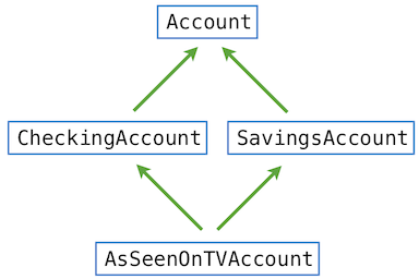
For a simple “diamond” shape like this, Python resolves names from left to right, then upwards. In this example, Python checks for an attribute name in the following classes, in order, until an attribute with that name is found:

AsSeenOnTVAccount, CheckingAccount, SavingsAccount, Account, object

There is no correct solution to the inheritance ordering problem, as there are cases in which we might prefer to give precedence to certain inherited classes over others. However, any programming language that supports multiple inheritance must select some ordering in a consistent way, so that users of the language can predict the behavior of their programs.

Further reading. Python resolves this name using a recursive algorithm called the C3 Method Resolution Ordering. The method resolution order of any class can be queried using the mro method on all classes.

>>> [c.__name__ for c in AsSeenOnTVAccount.mro()]
['AsSeenOnTVAccount', 'CheckingAccount', 'SavingsAccount', 'Account', 'object']

The precise algorithm for finding method resolution orderings is not a topic for this text, but is described by Python’s primary author with a reference to the original paper.

2.5.8 The Role of Objects

The Python object system is designed to make data abstraction and message passing both convenient and flexible. The specialized syntax of classes, methods, inheritance, and dot expressions all enable us to formalize the object metaphor in our programs, which improves our ability to organize large programs.

In particular, we would like our object system to promote a separation of concerns among the different aspects of the program. Each object in a program encapsulates and manages some part of the program’s state, and each class statement defines the functions that implement some part of the program’s overall logic. Abstraction barriers enforce the boundaries between different aspects of a large program.

Object-oriented programming is particularly well-suited to programs that model systems that have separate but interacting parts. For instance, different users interact in a social network, different characters interact in a game, and different shapes interact in a physical simulation. When representing such systems, the objects in a program often map naturally onto objects in the system being modeled, and classes represent their types and relationships.

On the other hand, classes may not provide the best mechanism for implementing certain abstractions. Functional abstractions provide a more natural metaphor for representing relationships between inputs and outputs. One should not feel compelled to fit every bit of logic in a program within a class, especially when defining independent functions for manipulating data is more natural. Functions can also enforce a separation of concerns.

Multi-paradigm languages such as Python allow programmers to match organizational paradigms to appropriate problems. Learning to identify when to introduce a new class, as opposed to a new function, in order to simplify or modularize a program, is an important design skill in software engineering that deserves careful attention.

2.6 Implementing Classes and Objects

When working in the object-oriented programming paradigm, we use the object metaphor to guide the organization of our programs. Most logic about how to represent and manipulate data is expressed within class declarations. In this section, we see that classes and objects can themselves be represented using just functions and dictionaries. The purpose of implementing an object system in this way is to illustrate that using the object metaphor does not require a special programming language. Programs can be object-oriented, even in programming languages that do not have a built-in object system.

In order to implement objects, we will abandon dot notation (which does require built-in language support), but create dispatch dictionaries that behave in much the same way as the elements of the built-in object system. We have already seen how to implement message-passing behavior through dispatch dictionaries. To implement an object system in full, we send messages between instances, classes, and base classes, all of which are dictionaries that contain attributes.

We will not implement the entire Python object system, which includes features that we have not covered in this text (e.g., meta-classes and static methods). We will focus instead on user-defined classes without multiple inheritance and without introspective behavior (such as returning the class of an instance). Our implementation is not meant to follow the precise specification of the Python type system. Instead, it is designed to implement the core functionality that enables the object metaphor.

2.6.1 Instances

We begin with instances. An instance has named attributes, such as the balance of an account, which can be set and retrieved. We implement an instance using a dispatch dictionary that responds to messages that “get” and “set” attribute values. Attributes themselves are stored in a local dictionary called attributes.

As we have seen previously in this chapter, dictionaries themselves are abstract data types. We implemented dictionaries with lists, we implemented lists with pairs, and we implemented pairs with functions. As we implement an object system in terms of dictionaries, keep in mind that we could just as well be implementing objects using functions alone.

To begin our implementation, we assume that we have a class implementation that can look up any names that are not part of the instance. We pass in a class to make_instance as the parameter cls.

>>> def make_instance(cls):
        """Return a new object instance, which is a dispatch dictionary."""
        def get_value(name):
            if name in attributes:
                return attributes[name]
            else:
                value = cls['get'](name)
                return bind_method(value, instance)
        def set_value(name, value):
            attributes[name] = value
        attributes = {}
        instance = {'get': get_value, 'set': set_value}
        return instance

The instance is a dispatch dictionary that responds to the messages get and set. The set message corresponds to attribute assignment in Python’s object system: all assigned attributes are stored directly within the object’s local attribute dictionary. In get, if name does not appear in the local attributesdictionary, then it is looked up in the class. If the value returned by cls is a function, it must be bound to the instance.

Bound method values. The get_value function in make_instance finds a named attribute in its class with get, then calls bind_method. Binding a method only applies to function values, and it creates a bound method value from a function value by inserting the instance as the first argument:

>>> def bind_method(value, instance):
        """Return a bound method if value is callable, or value otherwise."""
        if callable(value):
            def method(*args):
                return value(instance, *args)
            return method
        else:
            return value

When a method is called, the first parameter self will be bound to the value of instance by this definition.

2.6.2 Classes

A class is also an object, both in Python’s object system and the system we are implementing here. For simplicity, we say that classes do not themselves have a class. (In Python, classes do have classes; almost all classes share the same class, called type.) A class can respond to get and set messages, as well as the new message:

>>> def make_class(attributes, base_class=None):
        """Return a new class, which is a dispatch dictionary."""
        def get_value(name):
            if name in attributes:
                return attributes[name]
            elif base_class is not None:
                return base_class['get'](name)
        def set_value(name, value):
            attributes[name] = value
        def new(*args):
            return init_instance(cls, *args)
        cls = {'get': get_value, 'set': set_value, 'new': new}
        return cls

Unlike an instance, the get function for classes does not query its class when an attribute is not found, but instead queries its base_class. No method binding is required for classes.

Initialization. The new function in make_class calls init_instance, which first makes a new instance, then invokes a method called __init__.

>>> def init_instance(cls, *args):
        """Return a new object with type cls, initialized with args."""
        instance = make_instance(cls)
        init = cls['get']('__init__')
        if init:
            init(instance, *args)
        return instance

This final function completes our object system. We now have instances, which set locally but fall back to their classes on get. After an instance looks up a name in its class, it binds itself to function values to create methods. Finally, classes can create new instances, and they apply their __init__ constructor function immediately after instance creation.

In this object system, the only function that should be called by the user is make_class. All other functionality is enabled through message passing. Similarly, Python’s object system is invoked via the class statement, and all of its other functionality is enabled through dot expressions and calls to classes.

2.6.3 Using Implemented Objects

We now return to use the bank account example from the previous section. Using our implemented object system, we will create an Account class, a CheckingAccount subclass, and an instance of each.

The Account class is created through a make_account_class function, which has structure similar to a class statement in Python, but concludes with a call to make_class.

>>> def make_account_class():
        """Return the Account class, which has deposit and withdraw methods."""
        interest = 0.02
        def __init__(self, account_holder):
            self['set']('holder', account_holder)
            self['set']('balance', 0)
        def deposit(self, amount):
            """Increase the account balance by amount and return the new balance."""
            new_balance = self['get']('balance') + amount
            self['set']('balance', new_balance)
            return self['get']('balance')
        def withdraw(self, amount):
            """Decrease the account balance by amount and return the new balance."""
            balance = self['get']('balance')
            if amount > balance:
                return 'Insufficient funds'
            self['set']('balance', balance - amount)
            return self['get']('balance')
        return make_class(locals())

The final call to locals returns a dictionary with string keys that contains the name-value bindings in the current local frame.

The Account class is finally instantiated via assignment.

>>> Account = make_account_class()

Then, an account instance is created via the new message, which requires a name to go with the newly created account.

>>> kirk_account = Account['new']('Kirk')

Then, get messages passed to kirk_account retrieve properties and methods. Methods can be called to update the balance of the account.

>>> kirk_account['get']('holder')
'Kirk'
>>> kirk_account['get']('interest')
0.02
>>> kirk_account['get']('deposit')(20)
20
>>> kirk_account['get']('withdraw')(5)
15

As with the Python object system, setting an attribute of an instance does not change the corresponding attribute of its class.

>>> kirk_account['set']('interest', 0.04)
>>> Account['get']('interest')
0.02

Inheritance. We can create a subclass CheckingAccount by overloading a subset of the class attributes. In this case, we change the withdraw method to impose a fee, and we reduce the interest rate.

>>> def make_checking_account_class():
        """Return the CheckingAccount class, which imposes a $1 withdrawal fee."""
        interest = 0.01
        withdraw_fee = 1
        def withdraw(self, amount):
            fee = self['get']('withdraw_fee')
            return Account['get']('withdraw')(self, amount + fee)
        return make_class(locals(), Account)

In this implementation, we call the withdraw function of the base class Account from the withdrawfunction of the subclass, as we would in Python’s built-in object system. We can create the subclass itself and an instance, as before.

>>> CheckingAccount = make_checking_account_class()
>>> jack_acct = CheckingAccount['new']('Spock')

Deposits behave identically, as does the constructor function. withdrawals impose the $1 fee from the specialized withdraw method, and interest has the new lower value from CheckingAccount.

>>> jack_acct['get']('interest')
0.01
>>> jack_acct['get']('deposit')(20)
20
>>> jack_acct['get']('withdraw')(5)
14

Our object system built upon dictionaries is quite similar in implementation to the built-in object system in Python. In Python, an instance of any user-defined class has a special attribute __dict__ that stores the local instance attributes for that object in a dictionary, much like our attributes dictionary. Python differs because it distinguishes certain special methods that interact with built-in functions to ensure that those functions behave correctly for arguments of many different types. Functions that operate on different types are the subject of the next section.

2.7 Object Abstraction

The object system allows programmers to build and use abstract data representations efficiently. It is also designed to allow multiple representations of abstract data to coexist in the same program.

A central concept in object abstraction is a generic function, which is a function that can accept values of multiple different types. We will consider three different techniques for implementing generic functions: shared interfaces, type dispatching, and type coercion. In the process of building up these concepts, we will also discover features of the Python object system that support the creation of generic functions.

2.7.1 String Conversion

To represent data effectively, an object value should behave like the kind of data it is meant to represent, including producing a string representation of itself. String representations of data values are especially important in an interactive language such as Python that automatically displays the string representation of the values of expressions in an interactive session.

String values provide a fundamental medium for communicating information among humans. Sequences of characters can be rendered on a screen, printed to paper, read aloud, converted to braille, or broadcast as Morse code. Strings are also fundamental to programming because they can represent Python expressions.

Python stipulates that all objects should produce two different string representations: one that is human-interpretable text and one that is a Python-interpretable expression. The constructor function for strings,str, returns a human-readable string. Where possible, the repr function returns a Python expression that evaluates to an equal object. The docstring for repr explains this property:

repr(object) -> string

Return the canonical string representation of the object.
For most object types, eval(repr(object)) == object.

The result of calling repr on the value of an expression is what Python prints in an interactive session.

>>> 12e12
12000000000000.0
>>> print(repr(12e12))
12000000000000.0

In cases where no representation exists that evaluates to the original value, Python typically produces a description surrounded by angled brackets.

>>> repr(min)
'<built-in function min>'

The str constructor often coincides with repr, but provides a more interpretable text representation in some cases. For instance, we see a difference between str and repr with dates.

>>> from datetime import date
>>> tues = date(2011, 9, 12)
>>> repr(tues)
'datetime.date(2011, 9, 12)'
>>> str(tues)
'2011-09-12'

Defining the repr function presents a new challenge: we would like it to apply correctly to all data types, even those that did not exist when repr was implemented. We would like it to be a generic or polymorphic function, one that can be applied to many (poly) different forms (morph) of data.

The object system provides an elegant solution in this case: the repr function always invokes a method called __repr__ on its argument.

>>> tues.__repr__()
'datetime.date(2011, 9, 12)'

By implementing this same method in user-defined classes, we can extend the applicability of repr to any class we create in the future. This example highlights another benefit of dot expressions in general, that they provide a mechanism for extending the domain of existing functions to new object types.

The str constructor is implemented in a similar manner: it invokes a method called __str__ on its argument.

>>> tues.__str__()
'2011-09-12'

These polymorphic functions are examples of a more general principle: certain functions should apply to multiple data types. Moreover, one way to create such a function is to use a shared attribute name with a different definition in each class.

2.7.2 Special Methods

In Python, certain special names are invoked by the Python interpreter in special circumstances. For instance, the __init__ method of a class is automatically invoked whenever an object is constructed. The __str__ method is invoked automatically when printing, and __repr__ is invoked in an interactive session to display values.

There are special names for many other behaviors in Python. Some of those used most commonly are described below.

True and false values. We saw previously that numbers in Python have a truth value; more specifically, 0 is a false value and all other numbers are true values. In fact, all objects in Python have a truth value. By default, objects of user-defined classes are considered to be true, but the special __bool__ method can be used to override this behavior. If an object defines the __bool__ method, then Python calls that method to determine its truth value.

As an example, suppose we want a bank account with 0 balance to be false. We can add a __bool__method to the Account class to create this behavior.

>>> Account.__bool__ = lambda self: self.balance != 0

We can call the bool constructor to see the truth value of an object, and we can use any object in a boolean context.

>>> bool(Account('Jack'))
False
>>> if not Account('Jack'):
        print('Jack has nothing')
Jack has nothing

Sequence operations. We have seen that we can call the len function to determine the length of a sequence.

>>> len('Go Bears!')
9

The len function invokes the __len__ method of its argument to determine its length. All built-in sequence types implement this method.

>>> 'Go Bears!'.__len__()
9

Python uses a sequence’s length to determine its truth value, if it does not provide a __bool__ method. Empty sequences are false, while non-empty sequences are true.

>>> bool('')
False
>>> bool([])
False
>>> bool('Go Bears!')
True

The __getitem__ method is invoked by the element selection operator, but it can also be invoked directly.

>>> 'Go Bears!'[3]
'B'
>>> 'Go Bears!'.__getitem__(3)
'B'

Callable objects. In Python, functions are first-class objects, so they can be passed around as data and have attributes like any other object. Python also allows us to define objects that can be “called” like functions by including a __call__ method. With this method, we can define a class that behaves like a higher-order function.

As an example, consider the following higher-order function, which returns a function that adds a constant value to its argument.

>>> def make_adder(n):
        def adder(k):
            return n + k
        return adder
>>> add_three = make_adder(3)
>>> add_three(4)
7

We can create an Adder class that defines a __call__ method to provide the same functionality.

>>> class Adder(object):
        def __init__(self, n):
            self.n = n
        def __call__(self, k):
            return self.n + k
>>> add_three_obj = Adder(3)
>>> add_three_obj(4)
7

Here, the Adder class behaves like the make_adder higher-order function, and the add_three_obj object behaves like the add_three function. We have further blurred the line between data and functions.

Arithmetic. Special methods can also define the behavior of built-in operators applied to user-defined objects. In order to provide this generality, Python follows specific protocols to apply each operator. For example, to evaluate expressions that contain the + operator, Python checks for special methods on both the left and right operands of the expression. First, Python checks for an __add__ method on the value of the left operand, then checks for an __radd__ method on the value of the right operand. If either is found, that method is invoked with the value of the other operand as its argument. Some examples are given in the following sections. For readers interested in further details, the Python documentation describes the exhaustive set of method names for operators. Dive into Python 3 has a chapter on special method names that describes how many of these special method names are used.

2.7.3 Multiple Representations

Abstraction barriers allow us to separate the use and representation of data. However, in large programs, it may not always make sense to speak of “the underlying representation” for a data type in a program. For one thing, there might be more than one useful representation for a data object, and we might like to design systems that can deal with multiple representations.

To take a simple example, complex numbers may be represented in two almost equivalent ways: in rectangular form (real and imaginary parts) and in polar form (magnitude and angle). Sometimes the rectangular form is more appropriate and sometimes the polar form is more appropriate. Indeed, it is perfectly plausible to imagine a system in which complex numbers are represented in both ways, and in which the functions for manipulating complex numbers work with either representation. We implement such a system below. As a side note, we are developing a system that performs arithmetic operations on complex numbers as a simple but unrealistic example of a program that uses generic operations. Acomplex number type is actually built into Python, but for this example we will implement our own.

The idea of allowing for multiple representations of data arises regularly. Large software systems are often designed by many people working over extended periods of time, subject to requirements that change over time. In such an environment, it is simply not possible for everyone to agree in advance on choices of data representation. In addition to the data-abstraction barriers that isolate representation from use, we need abstraction barriers that isolate different design choices from each other and permit different choices to coexist in a single program.

We will begin our implementation at the highest level of abstraction and work towards concrete representations. A Complex number is a Number, and numbers can be added or multiplied together. How numbers can be added or multiplied is abstracted by the method names add and mul.

>>> class Number:
        def __add__(self, other):
            return self.add(other)
        def __mul__(self, other):
            return self.mul(other)

This class requires that Number objects have add and mul methods, but does not define them. Moreover, it does not have an __init__ method. The purpose of Number is not to be instantiated directly, but instead to serve as a superclass of various specific number classes. Our next task is to define add and mul appropriately for complex numbers.

A complex number can be thought of as a point in two-dimensional space with two orthogonal axes, the real axis and the imaginary axis. From this perspective, the complex number c = real + imag * i(where i * i = -1) can be thought of as the point in the plane whose horizontal coordinate is real and whose vertical coordinate is imag. Adding complex numbers involves adding their respective real and imag coordinates.

When multiplying complex numbers, it is more natural to think in terms of representing a complex number in polar form, as a magnitude and an angle. The product of two complex numbers is the vector obtained by stretching one complex number by a factor of the length of the other, and then rotating it through the angle of the other.

The Complex class inherits from Number and describes arithmetic for complex numbers.

>>> class Complex(Number):
        def add(self, other):
            return ComplexRI(self.real + other.real, self.imag + other.imag)
        def mul(self, other):
            magnitude = self.magnitude * other.magnitude
            return ComplexMA(magnitude, self.angle + other.angle)

This implementation assumes that two classes exist for complex numbers, corresponding to their two natural representations:

• ComplexRI constructs a complex number from real and imaginary parts.
• ComplexMA constructs a complex number from a magnitude and angle.

Interfaces. Object attributes, which are a form of message passing, allows different data types to respond to the same message in different ways. A shared set of messages that elicit similar behavior from different classes is a powerful method of abstraction. An interface is a set of shared attribute names, along with a specification of their behavior. In the case of complex numbers, the interface needed to implement arithmetic consists of four attributes: real, imag, magnitude, and angle.

For complex arithmetic to be correct, these attributes must be consistent. That is, the rectangular coordinates (real, imag) and the polar coordinates (magnitude, angle) must describe the same point on the complex plane. The Complex class implicitly defines this interface by determining how these attributes are used to add and mul complex numbers.

Properties. The requirement that two or more attribute values maintain a fixed relationship with each other is a new problem. One solution is to store attribute values for only one representation and compute the other representation whenever it is needed.

Python has a simple feature for computing attributes on the fly from zero-argument functions. The @property decorator allows functions to be called without call expression syntax (parentheses following an expression). The ComplexRI class stores real and imag attributes and computes magnitude and angleon demand.

>>> from math import atan2
>>> class ComplexRI(Complex):
        def __init__(self, real, imag):
            self.real = real
            self.imag = imag
        @property
        def magnitude(self):
            return (self.real ** 2 + self.imag ** 2) ** 0.5
        @property
        def angle(self):
            return atan2(self.imag, self.real)
        def __repr__(self):
            return 'ComplexRI({0:g}, {1:g})'.format(self.real, self.imag)

As a result of this implementation, all four attributes needed for complex arithmetic can be accessed without any call expressions, and changes to real or imag are reflected in the magnitude and angle.

>>> ri = ComplexRI(5, 12)
>>> ri.real
5
>>> ri.magnitude
13.0
>>> ri.real = 9
>>> ri.real
9
>>> ri.magnitude
15.0

Similarly, the ComplexMA class stores magnitude and angle, but computes real and imag whenever those attributes are looked up.

>>> from math import sin, cos, pi
>>> class ComplexMA(Complex):
        def __init__(self, magnitude, angle):
            self.magnitude = magnitude
            self.angle = angle
        @property
        def real(self):
            return self.magnitude * cos(self.angle)
        @property
        def imag(self):
            return self.magnitude * sin(self.angle)
        def __repr__(self):
            return 'ComplexMA({0:g}, {1:g} * pi)'.format(self.magnitude, self.angle/pi)

Changes to the magnitude or angle are reflected immediately in the real and imag attributes.

>>> ma = ComplexMA(2, pi/2)
>>> ma.imag
2.0
>>> ma.angle = pi
>>> ma.real
-2.0

Our implementation of complex numbers is now complete. Either class implementing complex numbers can be used for either argument in either arithmetic function in Complex.

>>> from math import pi
>>> ComplexRI(1, 2) + ComplexMA(2, pi/2)
ComplexRI(1, 4)
>>> ComplexRI(0, 1) * ComplexRI(0, 1)
ComplexMA(1, 1 * pi)

The interface approach to encoding multiple representations has appealing properties. The class for each representation can be developed separately; they must only agree on the names of the attributes they share, as well as any behavior conditions for those attributes. The interface is also additive. If another programmer wanted to add a third representation of complex numbers to the same program, they would only have to create another class with the same attributes.

Multiple representations of data are closely related to the idea of data abstraction with which we began this chapter. Using data abstraction, we were able to change the implementation of a data type without changing the meaning of the program. With interfaces and message passing, we can have multiple different representations within the same program. In both cases, a set of names and corresponding behavior conditions define the abstraction that enables this flexibility.

2.7.4 Generic Functions

Generic functions are methods or functions that apply to arguments of different types. We have seen many examples already. The Complex.add method is generic, because it can take either a ComplexRI or ComplexMA as the value for other. This flexibility was gained by ensuring that both ComplexRI and ComplexMA share an interface. Using interfaces and message passing is only one of several methods used to implement generic functions. We will consider two others in this section: type dispatching and type coercion.

Suppose that, in addition to our complex number classes, we implement a Rational class to represent fractions exactly. The add and mul methods express the same computations as the add_rational andmul_rational functions from earlier in the chapter.

>>> from fractions import gcd
>>> class Rational(Number):
        def __init__(self, numer, denom):
            g = gcd(numer, denom)
            self.numer = numer // g
            self.denom = denom // g
        def __repr__(self):
            return 'Rational({0}, {1})'.format(self.numer, self.denom)
        def add(self, other):
            nx, dx = self.numer, self.denom
            ny, dy = other.numer, other.denom
            return Rational(nx * dy + ny * dx, dx * dy)
        def mul(self, other):
            numer = self.numer * other.numer
            denom = self.denom * other.denom
            return Rational(numer, denom)

We have implemented the interface of the Number superclass by including add and mul methods. As a result, we can add and multiply rational numbers using familiar operators.

>>> Rational(2, 5) + Rational(1, 10)
Rational(1, 2)
>>> Rational(1, 4) * Rational(2, 3)
Rational(1, 6)

However, we cannot yet add a rational number to a complex number, although in mathematics such a combination is well-defined. We would like to introduce this cross-type operation in some carefully controlled way, so that we can support it without seriously violating our abstraction barriers. There is a tension between the outcomes we desire: we would like to be able to add a complex number to a rational number, and we would like to do so using a generic __add__ method that does the right thing with all numeric types. At the same time, we would like to separate the concerns of complex numbers and rational numbers whenever possible, in order to maintain a modular program.

Type dispatching. One way to implement cross-type operations is to select behavior based on the types of the arguments to a function or method. The idea of type dispatching is to write functions that inspect the type of arguments they receive, then execute code that is appropriate for those types.

The built-in function isinstance takes an object and a class. It returns true if the object has a class that either is or inherits from the given class.

>>> c = ComplexRI(1, 1)
>>> isinstance(c, ComplexRI)
True
>>> isinstance(c, Complex)
True
>>> isinstance(c, ComplexMA)
False

A simple example of type dispatching is an is_real function that uses a different implementation for each type of complex number.

>>> def is_real(c):
        """Return whether c is a real number with no imaginary part."""
        if isinstance(c, ComplexRI):
            return c.imag == 0
        elif isinstance(c, ComplexMA):
            return c.angle % pi == 0
>>> is_real(ComplexRI(1, 1))
False
>>> is_real(ComplexMA(2, pi))
True

Type dispatching is not always performed using isinstance. For arithmetic, we will give a type_tagattribute to Rational and Complex instances that has a string value. When two values x and y have the same type_tag, then we can combine them directly with x.add(y). If not, we need a cross-type operation.

>>> Rational.type_tag = 'rat'
>>> Complex.type_tag = 'com'
>>> Rational(2, 5).type_tag == Rational(1, 2).type_tag
True
>>> ComplexRI(1, 1).type_tag == ComplexMA(2, pi/2).type_tag
True
>>> Rational(2, 5).type_tag == ComplexRI(1, 1).type_tag
False

To combine complex and rational numbers, we write functions that rely on both of their representations simultaneously. Below, we rely on the fact that a Rational can be converted approximately to a floatvalue that is a real number. The result can be combined with a complex number.

>>> def add_complex_and_rational(c, r):
        return ComplexRI(c.real + r.numer/r.denom, c.imag)

Multiplication involves a similar conversion. In polar form, a real number in the complex plane always has a positive magnitude. The angle 0 indicates a positive number. The angle pi indicates a negative number.

>>> def mul_complex_and_rational(c, r):
        r_magnitude, r_angle = r.numer/r.denom, 0
        if r_magnitude < 0:
            r_magnitude, r_angle = -r_magnitude, pi
        return ComplexMA(c.magnitude * r_magnitude, c.angle + r_angle)

Both addition and multiplication are commutative, so swapping the argument order can use the same implementations of these cross-type operations.

>>> def add_rational_and_complex(r, c):
        return add_complex_and_rational(c, r)
>>> def mul_rational_and_complex(r, c):
        return mul_complex_and_rational(c, r)

The role of type dispatching is to ensure that these cross-type operations are used at appropriate times. Below, we rewrite the Number superclass to use type dispatching for its __add__ and __mul__ methods.

We use the type_tag attribute to distinguish types of arguments. One could directly use the built-in isinstance method as well, but tags simplify the implementation. Using type tags also illustrates that type dispatching is not necessarily linked to the Python object system, but instead a general technique for creating generic functions over heterogeneous domains.

The __add__ method considers two cases. First, if two arguments have the same type tag, then it assumes that add method of the first can take the second as an argument. Otherwise, it checks whether a dictionary of cross-type implementations, called adders, contains a function that can add arguments of those type tags. If there is such a function, the cross_apply method finds and applies it. The __mul__method has a similar structure.

>>> class Number:
        def __add__(self, other):
            if self.type_tag == other.type_tag:
                return self.add(other)
            elif (self.type_tag, other.type_tag) in self.adders:
                return self.cross_apply(other, self.adders)
        def __mul__(self, other):
            if self.type_tag == other.type_tag:
                return self.mul(other)
            elif (self.type_tag, other.type_tag) in self.multipliers:
                return self.cross_apply(other, self.multipliers)
        def cross_apply(self, other, cross_fns):
            cross_fn = cross_fns[(self.type_tag, other.type_tag)]
            return cross_fn(self, other)
        adders = {("com", "rat"): add_complex_and_rational,
                  ("rat", "com"): add_rational_and_complex}
        multipliers = {("com", "rat"): mul_complex_and_rational,
                       ("rat", "com"): mul_rational_and_complex}

In this new definition of the Number class, all cross-type implementations are indexed by pairs of type tags in the adders and multipliers dictionaries.

This dictionary-based approach to type dispatching is extensible. New subclasses of Number could install themselves into the system by declaring a type tag and adding cross-type operations to Number.addersand Number.multipliers. They could also define their own adders and multipliers in a subclass.

While we have introduced some complexity to the system, we can now mix types in addition and multiplication expressions.

>>> ComplexRI(1.5, 0) + Rational(3, 2)
ComplexRI(3, 0)
>>> Rational(-1, 2) * ComplexMA(4, pi/2)
ComplexMA(2, 1.5 * pi)

Coercion. In the general situation of completely unrelated operations acting on completely unrelated types, implementing explicit cross-type operations, cumbersome though it may be, is the best that one can hope for. Fortunately, we can sometimes do better by taking advantage of additional structure that may be latent in our type system. Often the different data types are not completely independent, and there may be ways by which objects of one type may be viewed as being of another type. This process is called coercion. For example, if we are asked to arithmetically combine a rational number with a complex number, we can view the rational number as a complex number whose imaginary part is zero. After doing so, we can use Complex.add and Complex.mul to combine them.

In general, we can implement this idea by designing coercion functions that transform an object of one type into an equivalent object of another type. Here is a typical coercion function, which transforms a rational number to a complex number with zero imaginary part:

>>> def rational_to_complex(r):
        return ComplexRI(r.numer/r.denom, 0)

The alternative definition of the Number class performs cross-type operations by attempting to coerce both arguments to the same type. The coercions dictionary indexes all possible coercions by a pair of type tags, indicating that the corresponding value coerces a value of the first type to a value of the second type.

It is not generally possible to coerce an arbitrary data object of each type into all other types. For example, there is no way to coerce an arbitrary complex number to a rational number, so there will be no such conversion implementation in the coercions dictionary.

The coerce method returns two values with the same type tag. It inspects the type tags of its arguments, compares them to entries in the coercions dictionary, and converts one argument to the type of the other using coerce_to. Only one entry in coercions is necessary to complete our cross-type arithmetic system, replacing the four cross-type functions in the type-dispatching version of Number.

>>> class Number:
        def __add__(self, other):
            x, y = self.coerce(other)
            return x.add(y)
        def __mul__(self, other):
            x, y = self.coerce(other)
            return x.mul(y)
        def coerce(self, other):
            if self.type_tag == other.type_tag:
                return self, other
            elif (self.type_tag, other.type_tag) in self.coercions:
                return (self.coerce_to(other.type_tag), other)
            elif (other.type_tag, self.type_tag) in self.coercions:
                return (self, other.coerce_to(self.type_tag))
        def coerce_to(self, other_tag):
            coercion_fn = self.coercions[(self.type_tag, other_tag)]
            return coercion_fn(self)
        coercions = {('rat', 'com'): rational_to_complex}

This coercion scheme has some advantages over the method of defining explicit cross-type operations. Although we still need to write coercion functions to relate the types, we need to write only one function for each pair of types rather than a different function for each set of types and each generic operation. What we are counting on here is the fact that the appropriate transformation between types depends only on the types themselves, not on the particular operation to be applied.

Further advantages come from extending coercion. Some more sophisticated coercion schemes do not just try to coerce one type into another, but instead may try to coerce two different types each into a third common type. Consider a rhombus and a rectangle: neither is a special case of the other, but both can be viewed as quadrilaterals. Another extension to coercion is iterative coercion, in which one data type is coerced into another via intermediate types. Consider that an integer can be converted into a real number by first converting it into a rational number, then converting that rational number into a real number. Chaining coercion in this way can reduce the total number of coercion functions that are required by a program.

Despite its advantages, coercion does have potential drawbacks. For one, coercion functions can lose information when they are applied. In our example, rational numbers are exact representations, but become approximations when they are converted to complex numbers.

Some programming languages have automatic coercion systems built in. In fact, early versions of Python had a __coerce__ special method on objects. In the end, the complexity of the built-in coercion system did not justify its use, and so it was removed. Instead, particular operators apply coercion to their arguments as needed.

C⚬MP⚬SING PR⚬GRAMS

• TEXT

• PROJECTS

• TUTOR

• ABOUT

Chapter 2Hide contents

2.1 Introduction

2.1.1 Native Data Types

2.2 Data Abstraction

2.2.1 Example: Rational Numbers

2.2.2 Pairs

2.2.3 Abstraction Barriers

2.2.4 The Properties of Data

2.3 Sequences

2.3.1 Lists

2.3.2 Sequence Iteration

2.3.3 Sequence Processing

2.3.4 Sequence Abstraction

2.3.5 Strings

2.3.6 Trees

2.3.7 Linked Lists

2.4 Mutable Data

2.4.1 The Object Metaphor

2.4.2 Sequence Objects

2.4.3 Dictionaries

2.4.4 Local State

2.4.5 The Benefits of Non-Local Assignment

2.4.6 The Cost of Non-Local Assignment

2.4.7 Iterators

2.4.8 Iterables

2.4.9 Built-in Iterators

2.4.10 Generators

2.4.11 Implementing Lists and Dictionaries

2.4.12 Dispatch Dictionaries

2.4.13 Propagating Constraints

2.5 Object-Oriented Programming

2.5.1 Objects and Classes

2.5.2 Defining Classes

2.5.3 Message Passing and Dot Expressions

2.5.4 Class Attributes

2.5.5 Inheritance

2.5.6 Using Inheritance

2.5.7 Multiple Inheritance

2.5.8 The Role of Objects

2.6 Implementing Classes and Objects

2.6.1 Instances

2.6.2 Classes

2.6.3 Using Implemented Objects

2.7 Object Abstraction

2.7.1 String Conversion

2.7.2 Special Methods

2.7.3 Multiple Representations

2.7.4 Generic Functions

2.8 Efficiency

2.8.1 Measuring Efficiency

2.8.2 Memoization

2.8.3 Orders of Growth

2.8.4 Example: Exponentiation

2.8.5 Growth Categories

2.9 Recursive Objects

2.9.1 Linked List Class

2.9.2 Tree Class

2.9.3 Sets

2.8 Efficiency

Decisions of how to represent and process data are often influenced by the efficiency of alternatives. Efficiency refers to the computational resources used by a representation or process, such as how much time and memory are required to compute the result of a function or represent an object. These amounts can vary widely depending on the details of an implementation.

2.8.1 Measuring Efficiency

Measuring exactly how long a program requires to run or how much memory it consumes is challenging, because the results depend upon many details of how a computer is configured. A more reliable way to characterize the efficiency of a program is to measure how many times some event occurs, such as a function call.

Let’s return to our first tree-recursive function, the fib function for computing numbers in the Fibonacci sequence.

>>> def fib(n):
        if n == 0:
            return 0
        if n == 1:
            return 1
        return fib(n-2) + fib(n-1)
>>> fib(5)
5

Consider the pattern of computation that results from evaluating fib(6), depicted below. To compute fib(5), we compute fib(3) and fib(4). To compute fib(3), we compute fib(1) and fib(2). In general, the evolved process looks like a tree. Each blue dot indicates a completed computation of a Fibonacci number in the traversal of this tree.

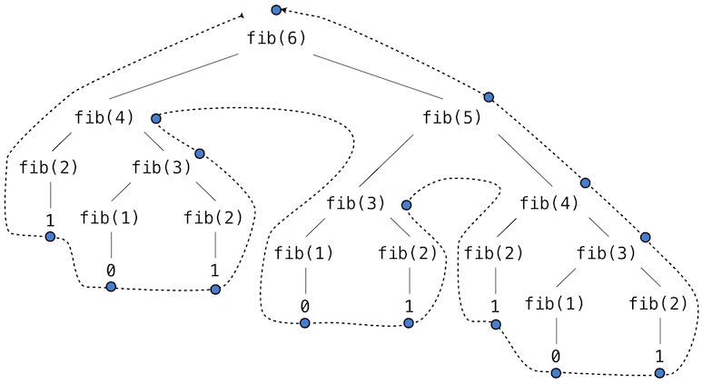
This function is instructive as a prototypical tree recursion, but it is a terribly inefficient way to compute Fibonacci numbers because it does so much redundant computation. The entire computation of fib(3)is duplicated.

We can measure this inefficiency. The higher-order count function returns an equivalent function to its argument that also maintains a call_count attribute. In this way, we can inspect just how many times fib is called.

>>> def count(f):
        def counted(*args):
            counted.call_count += 1
            return f(*args)
        counted.call_count = 0
        return counted

By counting the number of calls to fib, we see that the calls required grows faster than the Fibonacci numbers themselves. This rapid expansion of calls is characteristic of tree-recursive functions.

>>> fib = count(fib)
>>> fib(19)
4181
>>> fib.call_count
13529

Space. To understand the space requirements of a function, we must specify generally how memory is used, preserved, and reclaimed in our environment model of computation. In evaluating an expression, the interpreter preserves all active environments and all values and frames referenced by those environments. An environment is active if it provides the evaluation context for some expression being evaluated. An environment becomes inactive whenever the function call for which its first frame was created finally returns.

For example, when evaluating fib, the interpreter proceeds to compute each value in the order shown previously, traversing the structure of the tree. To do so, it only needs to keep track of those nodes that are above the current node in the tree at any point in the computation. The memory used to evaluate the rest of the branches can be reclaimed because it cannot affect future computation. In general, the space required for tree-recursive functions will be proportional to the maximum depth of the tree.

The diagram below depicts the environment created by evaluating fib(3). In the process of evaluating the return expression for the initial application of fib, the expression fib(n-2) is evaluated, yielding a value of 0. Once this value is computed, the corresponding environment frame (grayed out) is no longer needed: it is not part of an active environment. Thus, a well-designed interpreter can reclaim the memory that was used to store this frame. On the other hand, if the interpreter is currently evaluating fib(n-1), then the environment created by this application of fib (in which n is 2) is active. In turn, the environment originally created to apply fib to 3 is active because its return value has not yet been computed.

def fib(n):
    if n == 0:
        return 0
    if n == 1:
        return 1
    return fib(n-2) + fib(n-1)

result = fib(2)

The higher-order count_frames function tracks open_count, the number of calls to the function f that have not yet returned. The max_count attribute is the maximum value ever attained by open_count, and it corresponds to the maximum number of frames that are ever simultaneously active during the course of computation.

>>> def count_frames(f):
        def counted(*args):
            counted.open_count += 1
            counted.max_count = max(counted.max_count, counted.open_count)
            result = f(*args)
            counted.open_count -= 1
            return result
        counted.open_count = 0
        counted.max_count = 0
        return counted
>>> fib = count_frames(fib)
>>> fib(19)
4181
>>> fib.open_count
0
>>> fib.max_count
19
>>> fib(24)
46368
>>> fib.max_count
24

To summarize, the space requirement of the fib function, measured in active frames, is one less than the input, which tends to be small. The time requirement measured in total recursive calls is larger than the output, which tends to be huge.

2.8.2 Memoization

Tree-recursive computational processes can often be made more efficient through memoization, a powerful technique for increasing the efficiency of recursive functions that repeat computation. A memoized function will store the return value for any arguments it has previously received. A second call to fib(25) would not re-compute the return value recursively, but instead return the existing one that has already been constructed.

Memoization can be expressed naturally as a higher-order function, which can also be used as a decorator. The definition below creates a cache of previously computed results, indexed by the arguments from which they were computed. The use of a dictionary requires that the argument to the memoized function be immutable.

>>> def memo(f):
        cache = {}
        def memoized(n):
            if n not in cache:
                cache[n] = f(n)
            return cache[n]
        return memoized

If we apply memo to the recursive computation of Fibonacci numbers, a new pattern of computation evolves, depicted below.

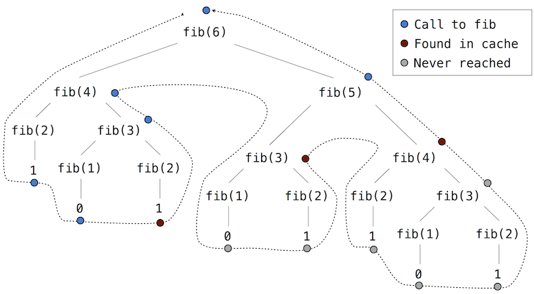
In this computation of fib(5), the results for fib(2) and fib(3) are reused when computing fib(4) on the right branch of the tree. As a result, much of the tree-recursive computation is not required at all.

Using count, we can see that the fib function is actually only called once for each unique input to fib.

>>> counted_fib = count(fib)
>>> fib  = memo(counted_fib)
>>> fib(19)
4181
>>> counted_fib.call_count
20
>>> fib(34)
5702887
>>> counted_fib.call_count
35

2.8.3 Orders of Growth

Processes can differ massively in the rates at which they consume the computational resources of space and time, as the previous examples illustrate. However, exactly determining just how much space or time will be used when calling a function is a very difficult task that depends upon many factors. A useful way to analyze a process is to categorize it along with a group of processes that all have similar requirements. A useful categorization is the order of growth of a process, which expresses in simple terms how the resource requirements of a process grow as a function of the input.

As an introduction to orders of growth, we will analyze the function count_factors below, which counts the number of integers that evenly divide an input n. The function attempts to divide n by every integer less than or equal to its square root. The implementation takes advantage of the fact that if $k$ divides $n$ and $k<\sqrt n$ , then there is another factor $j=n/ k$ such that $j > \sqrt n$.

from math import sqrt
def count_factors(n):
    sqrt_n = sqrt(n)
    k, factors = 1, 0
    while k < sqrt_n:
        if n % k == 0:
            factors += 2
        k += 1
    if k * k == n:
        factors += 1
    return factors

result = count_factors(576)

How much time is required to evaluate count_factors? The exact answer will vary on different machines, but we can make some useful general observations about the amount of computation involved. The total number of times this process executes the body of the while statement is the greatest integer less than $\sqrt n$. The statements before and after this while statement are executed exactly once. So, the total number of statements executed is $w \cdot {\sqrt n} + v$, where $w$ is the number of statements in the while body and $v$ is the number of statements outside of the while statement. Although it isn’t exact, this formula generally characterizes how much time will be required to evaluate count_factors as a function of the input n.

A more exact description is difficult to obtain. The constants $w$ and $v$ are not constant at all, because the assignment statements to factors are sometimes executed but sometimes not. An order of growth analysis allows us to gloss over such details and instead focus on the general shape of growth. In particular, the order of growth for count_factors expresses in precise terms that the amount of time required to compute count_factors(n) scales at the rate $\sqrt n $, within a margin of some constant factors.

Theta Notation. Let be a parameter that measures the size of the input to some process, and let $R(n)$ be the amount of some resource that the process requires for an input of size $n$. In our previous examples we took $n$ to be the number for which a given function is to be computed, but there are other possibilities. For instance, if our goal is to compute an approximation to the square root of a number, we might take $n$ to be the number of digits of accuracy required.

$ R(n)$ might measure the amount of memory used, the number of elementary machine steps performed, and so on. In computers that do only a fixed number of steps at a time, the time required to evaluate an expression will be proportional to the number of elementary steps performed in the process of evaluation.

We say that $R(n)$ has order of growth $\Theta (f(n))$, written $R(n) = \Theta (f(n))$ (pronounced “theta of $f(n)$”), if there are positive constants $k_1$ and $k_2$ independent of $n$ such that

$$k_1 \cdot f(n) \le R(n) \le k_2 \cdot f(n)$$

for any value of $n$ larger than some minimum $m$. In other words, for large $n$, the value $R(n)$ is always sandwiched between two values that both scale with $f(n)$:

• A lower bound $k_1 \cdot f(n)$ and
• An upper bound $k_2 \cdot f(n)$

We can apply this definition to show that the number of steps required to evaluate count_factors(n)grows as $\Theta (\sqrt n)$ by inspecting the function body.

First, we choose $k_1 = 1$ and $m=0$, so that the lower bound states that count_factors(n) requires at least $1 \cdot \sqrt n$ steps for any $n > 0$. There are at least 4 lines executed outside of the while statement, each of which takes at least 1 step to execute. There are at least two lines executed within the whilebody, along with the while header itself. All of these require at least one step. The while body is evaluated at least $\sqrt n - 1$ times. Composing these lower bounds, we see that the process requires at least $4 + 3 \cdot \sqrt n - 1$ steps, which is always larger than $k_1 \cdot \sqrt n$.

Second, we can verify the upper bound. We assume that any single line in the body of count_factorsrequires at most p steps. This assumption isn’t true for every line of Python, but does hold in this case. Then, evaluating count_factors(n) can require at most $p \cdot (5+4\sqrt n)$, because there are 5 lines outside of the while statement and 4 within (including the header). This upper bound holds even if every if header evaluates to true. Finally, if we choose $k_2 = 5p$, then the steps required is always smaller than $k_2 \cdot \sqrt n$. Our argument is complete.

2.8.4 Example: Exponentiation

Consider the problem of computing the exponential of a given number. We would like a function that takes as arguments a base b and a positive integer exponent n and computes bnbn. One way to do this is via the recursive definition

$$\begin {align} b^n &= b \cdot b^{n-1} \\ b^0 &= 1 \end {align}$$

which translates readily into the recursive function

>>> def exp(b, n):
        if n == 0:
            return 1
        return b * exp(b, n-1)

This is a linear recursive process that requires Θ(n)Θ(n) steps and Θ(n)Θ(n) space. Just as with factorial, we can readily formulate an equivalent linear iteration that requires a similar number of steps but constant space.

>>> def exp_iter(b, n):
        result = 1
        for _ in range(n):
            result = result * b
        return result

We can compute exponentials in fewer steps by using successive squaring. For instance, rather than computing $b^8$ as

$$b\cdot(b\cdot(b\cdot(b\cdot(b\cdot(b\cdot(b\cdot b)))))))$$

we can compute it using three multiplications:

$$\begin {align} b^2 &= b \cdot b \\ b^4 &= b^2 \cdot b^2 \\ b^8 &= b^4 \cdot b^4 \end {align}$$

This method works fine for exponents that are powers of 2. We can also take advantage of successive squaring in computing exponentials in general if we use the recursive rule

$$b^n= \left\{ \begin{array}{c} ( b^{\frac{n}{2}})^2 ~~~~~~if~n ~ is~even\\ b \cdot b^{n-1}~~~~~if~n ~ is~odd \end{array} \right.$$

We can express this method as a recursive function as well:

>>> def square(x):
        return x*x
>>> def fast_exp(b, n):
        if n == 0:
            return 1
        if n % 2 == 0:
            return square(fast_exp(b, n//2))
        else:
            return b * fast_exp(b, n-1)
>>> fast_exp(2, 100)
1267650600228229401496703205376

The process evolved by fast_exp grows logarithmically with n in both space and number of steps. To see this, observe that computing $b^{2n}$ using fast_exp requires only one more multiplication than computing $b^n$. The size of the exponent we can compute therefore doubles (approximately) with every new multiplication we are allowed. Thus, the number of multiplications required for an exponent of ngrows about as fast as the logarithm of n base 2. The process has $\Theta(\log n)$ growth. The difference between $\Theta(\log n)$ growth and $\Theta( n)$ growth becomes striking as nn becomes large. For example, fast_exp for n of 1000 requires only 14 multiplications instead of 1000.

2.8.5 Growth Categories

Orders of growth are designed to simplify the analysis and comparison of computational processes. Many different processes can all have equivalent orders of growth, which indicates that they scale in similar ways. It is an essential skill of a computer scientist to know and recognize common orders of growth and identify processes of the same order.

Constants. Constant terms do not affect the order of growth of a process. So, for instance, $\Theta( n)$ and $\Theta(500 \cdot n)$ are the same order of growth. This property follows from the definition of theta notation, which allows us to choose arbitrary constants $k_1$ and $k_2$ (such as $\frac{1}{500}$) for the upper and lower bounds. For simplicity, constants are always omitted from orders of growth.

Logarithms. The base of a logarithm does not affect the order of growth of a process. For instance, $\log_2 n$ and $\log_{10} n$ are the same order of growth. Changing the base of a logarithm is equivalent to multiplying by a constant factor.

Nesting. When an inner computational process is repeated for each step in an outer process, then the order of growth of the entire process is a product of the number of steps in the outer and inner processes.

For example, the function overlap below computes the number of elements in list a that also appear in list b.

>>> def overlap(a, b):
        count = 0
        for item in a:
            if item in b:
                count += 1
        return count
>>> overlap([1, 3, 2, 2, 5, 1], [5, 4, 2])
3

The in operator for lists requires $\Theta( n)$ time, where nn is the length of the list b. It is applied $\Theta( m)$ times, where mm is the length of the list a. The item in b expression is the inner process, and the for item in a loop is the outer process. The total order of growth for this function is $\Theta(m \cdot n)$.

Lower-order terms. As the input to a process grows, the fastest growing part of a computation dominates the total resources used. Theta notation captures this intuition. In a sum, all but the fastest growing term can be dropped without changing the order of growth.

For instance, consider the one_more function that returns how many elements of a list a are one more than some other element of a. That is, in the list [3, 14, 15, 9], the element 15 is one more than 14, so one_more will return 1.

>>> def one_more(a):
        return overlap([x-1 for x in a], a)
>>> one_more([3, 14, 15, 9])
1

There are two parts to this computation: the list comprehension and the call to overlap. For a list a of length nn, list comprehension requires $\Theta( n)$ steps, while the call to overlap requires $\Theta( n^2)$ steps. The sum of steps is $\Theta(n+n^2)$, but this is not the simplest way of expressing the order of growth.

$\Theta(n^2+k \cdot n)$ and $\Theta (n^2)$ are equivalent for any constant $k$ because the $n^2$ term will eventually dominate the total for any $k$. The fact that bounds must hold only for $n$ greater than some minimum $m$ establishes this equivalence. For simplicity, lower-order terms are always omitted from orders of growth, and so we will never see a sum within a theta expression.

Common categories. Given these equivalence properties, a small set of common categories emerge to describe most computational processes. The most common are listed below from slowest to fastest growth, along with descriptions of the growth as the input increases. Examples for each category follow.

Category	Theta Notation	Growth Description	Example
Constant	$\Theta (1)$	Growth is independent of the input	abs
Logarithmic	$\Theta (\log n)$	Multiplying input increments resources	fast_exp
Linear	$\Theta (n) $	Incrementing input increments resources	exp
Quadratic	$\Theta (n^2) $	Incrementing input adds n resources	one_more
Exponential	$\Theta (b^n) $	Incrementing input multiplies resources	fib

Other categories exist, such as the $\Theta (\sqrt n)$ growth of count_factors. However, these categories are particularly common.

Exponential growth describes many different orders of growth, because changing the base $b$ does affect the order of growth. For instance, the number of steps in our tree-recursive Fibonacci computation fibgrows exponentially in its input $n$. In particular, one can show that the nth Fibonacci number is the closest integer to

$$\frac {\phi ^{n-2}}{\sqrt 5}$$

where $\phi$ is the golden ratio:

$$\phi = \frac{1+ \sqrt 5}{2} \approx 1.6180$$

We also stated that the number of steps scales with the resulting value, and so the tree-recursive process requires $\Theta (\phi ^n)$ steps, a function that grows exponentially with $n$.

2.9 Recursive Objects

Objects can have other objects as attribute values. When an object of some class has an attribute value of that same class, it is a recursive object.

2.9.1 Linked List Class

A linked list, introduced earlier in this chapter, is composed of a first element and the rest of the list. The rest of a linked list is itself a linked list — a recursive definition. The empty list is a special case of a linked list that has no first element or rest. A linked list is a sequence: it has a finite length and supports element selection by index.

We can now implement a class with the same behavior. In this version, we will define its behavior using special method names that allow our class to work with the built-in len function and element selection operator (square brackets or operator.getitem) in Python. These built-in functions invoke special method names of a class: length is computed by __len__ and element selection is computed by __getitem__. The empty linked list is represented by an empty tuple, which has length 0 and no elements.

>>> class Link:
        """A linked list with a first element and the rest."""
        empty = ()
        def __init__(self, first, rest=empty):
            assert rest is Link.empty or isinstance(rest, Link)
            self.first = first
            self.rest = rest
        def __getitem__(self, i):
            if i == 0:
                return self.first
            else:
                return self.rest[i-1]
        def __len__(self):
            return 1 + len(self.rest)
>>> s = Link(3, Link(4, Link(5)))
>>> len(s)
3
>>> s[1]
4

The definitions of __len__ and __getitem__ are in fact recursive. The built-in Python function len invokes a method called __len__ when applied to a user-defined object argument. Likewise, the element selection operator invokes a method called __getitem__. Thus, bodies of these two methods will call themselves indirectly. For __len__, the base case is reached when self.rest evaluates to the empty tuple, Link.empty, which has a length of 0.

The built-in isinstance function returns whether the first argument has a type that is or inherits from the second argument. isinstance(rest, Link) is true if rest is a Link instance or an instance of some sub-class of Link.

Our implementation is complete, but an instance of the Link class is currently difficult to inspect. To help with debugging, we can also define a function to convert a Link to a string expression.

>>> def link_expression(s):
        """Return a string that would evaluate to s."""
        if s.rest is Link.empty:
            rest = ''
        else:
            rest = ', ' + link_expression(s.rest)
        return 'Link({0}{1})'.format(s.first, rest)
>>> link_expression(s)
'Link(3, Link(4, Link(5)))'

This way of displaying an Link is so convenient that we would like to use it whenever an Link instance is displayed. We can ensure this behavior by setting the link_expression function as the value of the special class attribute __repr__. Python displays instances of user-defined classes by invoking their __repr__ method.

>>> Link.__repr__ = link_expression
>>> s
Link(3, Link(4, Link(5)))

The Link class has the closure property. Just as an element of a list can itself be a list, a Link can contain a Link as its first element.

>>> s_first = Link(s, Link(6))
>>> s_first
Link(Link(3, Link(4, Link(5))), Link(6))

The s_first linked list has only two elements, but its first element is a linked list with three elements.

>>> len(s_first)
2
>>> len(s_first[0])
3
>>> s_first[0][2]
5

Recursive functions are particularly well-suited to manipulate linked lists. For instance, the recursive extend_link function builds a linked list containing the elements of one Link instance s followed by the elements of another Link instance t. Installing this function as the __add__ method of the Link class emulates the addition behavior of a built-in list.

>>> def extend_link(s, t):
        if s is Link.empty:
            return t
        else:
            return Link(s.first, extend_link(s.rest, t))
>>> extend_link(s, s)
Link(3, Link(4, Link(5, Link(3, Link(4, Link(5))))))
>>> Link.__add__ = extend_link
>>> s + s
Link(3, Link(4, Link(5, Link(3, Link(4, Link(5))))))

Rather than list comprehensions, one linked list can be generated from another using two higher-order functions: map_link and filter_link. The map_link function defined below applies a function f to each element of a linked list s and constructs a linked list containing the results.

>>> def map_link(f, s):
        if s is Link.empty:
            return s
        else:
            return Link(f(s.first), map_link(f, s.rest))
>>> map_link(square, s)
Link(9, Link(16, Link(25)))

The filter_link function returns a linked list containing all elements of a linked list s for which f returns a true value. The combination of map_link and filter_link can express the same logic as a list comprehension.

>>> def filter_link(f, s):
        if s is Link.empty:
            return s
        else:
            filtered = filter_link(f, s.rest)
            if f(s.first):
                return Link(s.first, filtered)
            else:
                return filtered
>>> odd = lambda x: x % 2 == 1
>>> map_link(square, filter_link(odd, s))
Link(9, Link(25))
>>> [square(x) for x in [3, 4, 5] if odd(x)]
[9, 25]

The join_link function recursively constructs a string that contains the elements of a linked list seperated by some separator string. The result is much more compact than the output of link_expression.

>>> def join_link(s, separator):
        if s is Link.empty:
            return ""
        elif s.rest is Link.empty:
            return str(s.first)
        else:
            return str(s.first) + separator + join_link(s.rest, separator)
>>> join_link(s, ", ")
'3, 4, 5'

Recursive Construction. Linked lists are particularly useful when constructing sequences incrementally, a situation that arises often in recursive computations.

The count_partitions function from Chapter 1 counted the number of ways to partition an integer nusing parts up to size m via a tree-recursive process. With sequences, we can also enumerate these partitions explicitly using a similar process.

We follow the same recursive analysis of the problem as we did while counting: partitioning n using integers up to m involves either

1. partitioning n-m using integers up to m, or
2. partitioning n using integers up to m-1.

For base cases, we find that 0 has an empty partition, while partitioning a negative integer or using parts smaller than 1 is impossible.

>>> def partitions(n, m):
        """Return a linked list of partitions of n using parts of up to m.
        Each partition is represented as a linked list.
        """
        if n == 0:
            return Link(Link.empty) # A list containing the empty partition
        elif n < 0 or m == 0:
            return Link.empty
        else:
            using_m = partitions(n-m, m)
            with_m = map_link(lambda s: Link(m, s), using_m)
            without_m = partitions(n, m-1)
            return with_m + without_m

In the recursive case, we construct two sublists of partitions. The first uses m, and so we add m to each element of the result using_m to form with_m.

The result of partitions is highly nested: a linked list of linked lists. Using join_link with appropriate separators, we can display the partitions in a human-readable manner.

>>> def print_partitions(n, m):
        lists = partitions(n, m)
        strings = map_link(lambda s: join_link(s, " + "), lists)
        print(join_link(strings, "\n"))
>>> print_partitions(6, 4)
4 + 2
4 + 1 + 1
3 + 3
3 + 2 + 1
3 + 1 + 1 + 1
2 + 2 + 2
2 + 2 + 1 + 1
2 + 1 + 1 + 1 + 1
1 + 1 + 1 + 1 + 1 + 1

2.9.2 Tree Class

Trees can also be represented by instances of user-defined classes, rather than nested instances of built-in sequence types. A tree is any data structure that has as an attribute a sequence of branches that are also trees.

Internal values. Previously, we defined trees in such a way that all values appeared at the leaves of the tree. It is also common to define trees that have internal values at the roots of each subtree. An internal value is called an label in the tree. The Tree class below represents such trees, in which each tree has a sequence of branches that are also trees.

>>> class Tree:
        def __init__(self, label, branches=()):
            self.label = label
            for branch in branches:
                assert isinstance(branch, Tree)
            self.branches = branches
        def __repr__(self):
            if self.branches:
                return 'Tree({0}, {1})'.format(self.label, repr(self.branches))
            else:
                return 'Tree({0})'.format(repr(self.label))
        def is_leaf(self):
            return not self.branches

The Tree class can represent, for instance, the values computed in an expression tree for the recursive implementation of fib, the function for computing Fibonacci numbers. The function fib_tree(n) below returns a Tree that has the nth Fibonacci number as its label and a trace of all previously computed Fibonacci numbers within its branches.

>>> def fib_tree(n):
        if n == 1:
            return Tree(0)
        elif n == 2:
            return Tree(1)
        else:
            left = fib_tree(n-2)
            right = fib_tree(n-1)
            return Tree(left.label + right.label, (left, right))
>>> fib_tree(5)
Tree(3, (Tree(1, (Tree(0), Tree(1))), Tree(2, (Tree(1), Tree(1, (Tree(0), Tree(1)))))))

Trees represented in this way are also processed using recursive functions. For example, we can sum the labels of a tree. As a base case, we return that an empty branch has no labels.

>>> def sum_labels(t):
        """Sum the labels of a Tree instance, which may be None."""
        return t.label + sum([sum_labels(b) for b in t.branches])
>>> sum_labels(fib_tree(5))
10

We can also apply memo to construct a Fibonacci tree, where repeated subtrees are only created once by the memoized version of fib_tree, but are used multiple times as branches of different larger trees.

>>> fib_tree = memo(fib_tree)
>>> big_fib_tree = fib_tree(35)
>>> big_fib_tree.label
5702887
>>> big_fib_tree.branches[0] is big_fib_tree.branches[1].branches[1]
True
>>> sum_labels = memo(sum_labels)
>>> sum_labels(big_fib_tree)
142587180

The amount of computation time and memory saved by memoization in these cases is substantial. Instead of creating 18,454,929 different instances of the Tree class, we now create only 35.

2.9.3 Sets

In addition to the list, tuple, and dictionary, Python has a fourth built-in container type called a set. Set literals follow the mathematical notation of elements enclosed in braces. Duplicate elements are removed upon construction. Sets are unordered collections, and so the printed ordering may differ from the element ordering in the set literal.

>>> s = {3, 2, 1, 4, 4}
>>> s
{1, 2, 3, 4}

Python sets support a variety of operations, including membership tests, length computation, and the standard set operations of union and intersection

>>> 3 in s
True
>>> len(s)
4
>>> s.union({1, 5})
{1, 2, 3, 4, 5}
>>> s.intersection({6, 5, 4, 3})
{3, 4}

In addition to union and intersection, Python sets support several other methods. The predicates isdisjoint, issubset, and issuperset provide set comparison. Sets are mutable, and can be changed one element at a time using add, remove, discard, and pop. Additional methods provide multi-element mutations, such as clear and update. The Python documentation for sets should be sufficiently intelligible at this point of the course to fill in the details.

Implementing sets. Abstractly, a set is a collection of distinct objects that supports membership testing, union, intersection, and adjunction. Adjoining an element and a set returns a new set that contains all of the original set’s elements along with the new element, if it is distinct. Union and intersection return the set of elements that appear in either or both sets, respectively. As with any data abstraction, we are free to implement any functions over any representation of sets that provides this collection of behaviors.

In the remainder of this section, we consider three different methods of implementing sets that vary in their representation. We will characterize the efficiency of these different representations by analyzing the order of growth of set operations. We will use our Link and Tree classes from earlier in this section, which allow for simple and elegant recursive solutions for elementary set operations.

Sets as unordered sequences. One way to represent a set is as a sequence in which no element appears more than once. The empty set is represented by the empty sequence. Membership testing walks recursively through the list.

>>> def empty(s):
        return s is Link.empty
>>> def set_contains(s, v):
        """Return True if and only if set s contains v."""
        if empty(s):
            return False
        elif s.first == v:
            return True
        else:
            return set_contains(s.rest, v)
>>> s = Link(4, Link(1, Link(5)))
>>> set_contains(s, 2)
False
>>> set_contains(s, 5)
True

This implementation of set_contains requires Θ(n)Θ(n) time on average to test membership of an element, where nn is the size of the set s. Using this linear-time function for membership, we can adjoin an element to a set, also in linear time.

>>> def adjoin_set(s, v):
        """Return a set containing all elements of s and element v."""
        if set_contains(s, v):
            return s
        else:
            return Link(v, s)
>>> t = adjoin_set(s, 2)
>>> t
Link(2, Link(4, Link(1, Link(5))))

In designing a representation, one of the issues with which we should be concerned is efficiency. Intersecting two sets set1 and set2 also requires membership testing, but this time each element of set1 must be tested for membership in set2, leading to a quadratic order of growth in the number of steps, Θ(n2)Θ(n2), for two sets of size nn.

>>> def intersect_set(set1, set2):
        """Return a set containing all elements common to set1 and set2."""
        return keep_if_link(set1, lambda v: set_contains(set2, v))
>>> intersect_set(t, apply_to_all_link(s, square))
Link(4, Link(1))

When computing the union of two sets, we must be careful not to include any element twice. The union_set function also requires a linear number of membership tests, creating a process that also includes Θ(n2)Θ(n2) steps.

>>> def union_set(set1, set2):
        """Return a set containing all elements either in set1 or set2."""
        set1_not_set2 = keep_if_link(set1, lambda v: not set_contains(set2, v))
        return extend_link(set1_not_set2, set2)
>>> union_set(t, s)
Link(2, Link(4, Link(1, Link(5))))

Sets as ordered sequences. One way to speed up our set operations is to change the representation so that the set elements are listed in increasing order. To do this, we need some way to compare two objects so that we can say which is bigger. In Python, many different types of objects can be compared using < and > operators, but we will concentrate on numbers in this example. We will represent a set of numbers by listing its elements in increasing order.

One advantage of ordering shows up in set_contains: In checking for the presence of an object, we no longer have to scan the entire set. If we reach a set element that is larger than the item we are looking for, then we know that the item is not in the set:

>>> def set_contains(s, v):
        if empty(s) or s.first > v:
            return False
        elif s.first == v:
            return True
        else:
            return set_contains(s.rest, v)
>>> u = Link(1, Link(4, Link(5)))
>>> set_contains(u, 0)
False
>>> set_contains(u, 4)
True

How many steps does this save? In the worst case, the item we are looking for may be the largest one in the set, so the number of steps is the same as for the unordered representation. On the other hand, if we search for items of many different sizes we can expect that sometimes we will be able to stop searching at a point near the beginning of the list and that other times we will still need to examine most of the list. On average we should expect to have to examine about half of the items in the set. Thus, the average number of steps required will be about n2n2. This is still Θ(n)Θ(n) growth, but it does save us some time in practice over the previous implementation.

We can obtain a more impressive speedup by re-implementing intersect_set. In the unordered representation, this operation required Θ(n2)Θ(n2) steps because we performed a complete scan of set2 for each element of set1. But with the ordered representation, we can use a more clever method. We iterate through both sets simultaneously, tracking an element e1 in set1 and e2 in set2. When e1 and e2 are equal, we include that element in the intersection.

Suppose, however, that e1 is less than e2. Since e2 is smaller than the remaining elements of set2, we can immediately conclude that e1 cannot appear anywhere in the remainder of set2 and hence is not in the intersection. Thus, we no longer need to consider e1; we discard it and proceed to the next element of set1. Similar logic advances through the elements of set2 when e2 < e1. Here is the function:

>>> def intersect_set(set1, set2):
        if empty(set1) or empty(set2):
            return Link.empty
        else:
            e1, e2 = set1.first, set2.first
            if e1 == e2:
                return Link(e1, intersect_set(set1.rest, set2.rest))
            elif e1 < e2:
                return intersect_set(set1.rest, set2)
            elif e2 < e1:
                return intersect_set(set1, set2.rest)
>>> intersect_set(s, s.rest)
Link(4, Link(5))

To estimate the number of steps required by this process, observe that in each step we shrink the size of at least one of the sets. Thus, the number of steps required is at most the sum of the sizes of set1 and set2, rather than the product of the sizes, as with the unordered representation. This is Θ(n)Θ(n) growth rather than Θ(n2)Θ(n2) — a considerable speedup, even for sets of moderate size. For example, the intersection of two sets of size 100 will take around 200 steps, rather than 10,000 for the unordered representation.

Adjunction and union for sets represented as ordered sequences can also be computed in linear time. These implementations are left as an exercise.

Sets as binary search trees. We can do better than the ordered-list representation by arranging the set elements in the form of a tree with exactly two branches. The entry of the root of the tree holds one element of the set. The entries within the left branch include all elements smaller than the one at the root. Entries in the right branch include all elements greater than the one at the root. The figure below shows some trees that represent the set {1, 3, 5, 7, 9, 11}. The same set may be represented by a tree in a number of different ways. In all binary search trees, all elements in the left branch be smaller than the entry at the root, and that all elements in the right subtree be larger.

The advantage of the tree representation is this: Suppose we want to check whether a value v is contained in a set. We begin by comparing v with entry. If v is less than this, we know that we need only search the left subtree; if v is greater, we need only search the right subtree. Now, if the tree is “balanced,” each of these subtrees will be about half the size of the original. Thus, in one step we have reduced the problem of searching a tree of size nn to searching a tree of size n2n2. Since the size of the tree is halved at each step, we should expect that the number of steps needed to search a tree grows as Θ(logn)Θ(log⁡n). For large sets, this will be a significant speedup over the previous representations. This set_contains function exploits the ordering structure of the tree-structured set.

>>> def set_contains(s, v):
        if s is None:
            return False
        elif s.entry == v:
            return True
        elif s.entry < v:
            return set_contains(s.right, v)
        elif s.entry > v:
            return set_contains(s.left, v)

Adjoining an item to a set is implemented similarly and also requires Θ(logn)Θ(log⁡n) steps. To adjoin a value v, we compare v with entry to determine whether v should be added to the right or to the left branch, and having adjoined v to the appropriate branch we piece this newly constructed branch together with the original entry and the other branch. If v is equal to the entry, we just return the node. If we are asked to adjoin v to an empty tree, we generate a Tree that has v as the entry and empty right and left branches. Here is the function:

>>> def adjoin_set(s, v):
        if s is None:
            return Tree(v)
        elif s.entry == v:
            return s
        elif s.entry < v:
            return Tree(s.entry, s.left, adjoin_set(s.right, v))
        elif s.entry > v:
            return Tree(s.entry, adjoin_set(s.left, v), s.right)
>>> adjoin_set(adjoin_set(adjoin_set(None, 2), 3), 1)
Tree(2, Tree(1), Tree(3))

Our claim that searching the tree can be performed in a logarithmic number of steps rests on the assumption that the tree is “balanced,” i.e., that the left and the right subtree of every tree have approximately the same number of elements, so that each subtree contains about half the elements of its parent. But how can we be certain that the trees we construct will be balanced? Even if we start with a balanced tree, adding elements with adjoin_set may produce an unbalanced result. Since the position of a newly adjoined element depends on how the element compares with the items already in the set, we can expect that if we add elements “randomly” the tree will tend to be balanced on the average.

But this is not a guarantee. For example, if we start with an empty set and adjoin the numbers 1 through 7 in sequence we end up with a highly unbalanced tree in which all the left subtrees are empty, so it has no advantage over a simple ordered list. One way to solve this problem is to define an operation that transforms an arbitrary tree into a balanced tree with the same elements. We can perform this transformation after every few adjoin_set operations to keep our set in balance.

Intersection and union operations can be performed on tree-structured sets in linear time by converting them to ordered lists and back. The details are left as an exercise.

Python set implementation. The set type that is built into Python does not use any of these representations internally. Instead, Python uses a representation that gives constant-time membership tests and adjoin operations based on a technique called hashing, which is a topic for another course. Built-in Python sets cannot contain mutable data types, such as lists, dictionaries, or other sets. To allow for nested sets, Python also includes a built-in immutable frozenset class that shares methods with the set class but excludes mutation methods and operators.

Chapter 3: Interpreting Computer Programs

3.1 Introduction

Chapters 1 and 2 describe the close connection between two fundamental elements of programming: functions and data. We saw how functions can be manipulated as data using higher-order functions. We also saw how data can be endowed with behavior using message passing and an object system. We have also studied techniques for organizing large programs, such as functional abstraction, data abstraction, class inheritance, and generic functions. These core concepts constitute a strong foundation upon which to build modular, maintainable, and extensible programs.

This chapter focuses on the third fundamental element of programming: programs themselves. A Python program is just a collection of text. Only through the process of interpretation do we perform any meaningful computation based on that text. A programming language like Python is useful because we can define an interpreter, a program that carries out Python’s evaluation and execution procedures. It is no exaggeration to regard this as the most fundamental idea in programming, that an interpreter, which determines the meaning of expressions in a programming language, is just another program.

To appreciate this point is to change our images of ourselves as programmers. We come to see ourselves as designers of languages, rather than only users of languages designed by others.

3.1.1 Programming Languages

Programming languages vary widely in their syntactic structures, features, and domain of application. Among general purpose programming languages, the constructs of function definition and function application are pervasive. On the other hand, powerful languages exist that do not include an object system, higher-order functions, assignment, or even control constructs such as while and forstatements. As an example of a powerful language with a minimal set of features, we will introduce the Scheme) programming language. The subset of Scheme introduced in this text does not allow mutable values at all.

In this chapter, we study the design of interpreters and the computational processes that they create when executing programs. The prospect of designing an interpreter for a general programming language may seem daunting. After all, interpreters are programs that can carry out any possible computation, depending on their input. However, many interpreters have an elegant common structure: two mutually recursive functions. The first evaluates expressions in environments; the second applies functions to arguments.

These functions are recursive in that they are defined in terms of each other: applying a function requires evaluating the expressions in its body, while evaluating an expression may involve applying one or more functions.

3.2 Functional Programming

The software running on any modern computer is written in a variety of programming languages. There are physical languages, such as the machine languages for particular computers. These languages are concerned with the representation of data and control in terms of individual bits of storage and primitive machine instructions. The machine-language programmer is concerned with using the given hardware to erect systems and utilities for the efficient implementation of resource-limited computations. High-level languages, erected on a machine-language substrate, hide concerns about the representation of data as collections of bits and the representation of programs as sequences of primitive instructions. These languages have means of combination and abstraction, such as function definition, that are appropriate to the larger-scale organization of software systems.

In this section, we introduce a high-level programming language that encourages a functional style. Our object of study, a subset of the Scheme language, employs a very similar model of computation to Python’s, but uses only expressions (no statements), specializes in symbolic computation, and employs only immutable values.

Scheme is a dialect of Lisp), the second-oldest programming language that is still widely used today (after Fortran). The community of Lisp programmers has continued to thrive for decades, and new dialects of Lisp such as Clojure have some of the fastest growing communities of developers of any modern programming language. To follow along with the examples in this text, you can download a Scheme interpreter.

3.2.1 Expressions

Scheme programs consist of expressions, which are either call expressions or special forms. A call expression consists of an operator expression followed by zero or more operand sub-expressions, as in Python. Both the operator and operand are contained within parentheses:

(quotient 10 2)

5

Scheme exclusively uses prefix notation. Operators are often symbols, such as + and *. Call expressions can be nested, and they may span more than one line:

(+ (* 3 5) (- 10 6))

19

(+ (* 3
      (+ (* 2 4)
         (+ 3 5)))
   (+ (- 10 7)
      6))

57

As in Python, Scheme expressions may be primitives or combinations. Number literals are primitives, while call expressions are combined forms that include arbitrary sub-expressions. The evaluation procedure of call expressions matches that of Python: first the operator and operand expressions are evaluated, and then the function that is the value of the operator is applied to the arguments that are the values of the operands.

The if expression in Scheme is a special form, meaning that while it looks syntactically like a call expression, it has a different evaluation procedure. The general form of an if expression is:

(if <predicate> <consequent> <alternative>)

To evaluate an if expression, the interpreter starts by evaluating the part of the expression. If the evaluates to a true value, the interpreter then evaluates the and returns its value. Otherwise it evaluates the and returns its value.

Numerical values can be compared using familiar comparison operators, but prefix notation is used in this case as well:

(>= 2 1)

true

The boolean values #t (or true) and #f (or false) in Scheme can be combined with boolean special forms, which have evaluation procedures similar to those in Python.

• (and ... ) The interpreter evaluates the expressions one at a time, in left-to-right order. If any evaluates to false, the value of the and expression is false, and the rest of the 's are not evaluated. If all‘s evaluate to true values, the value of the andexpression is the value of the last one.
• (or ... ) The interpreter evaluates the expressions one at a time, in left-to-right order. If any evaluates to a true value, that value is returned as the value of the orexpression, and the rest of the 's are not evaluated. If all‘s evaluate to false, the value of the or expression is false.
• (not ) The value of a not expression is true when the expression ` evaluates tofalse, andfalse` otherwise.

3.2.2 Definitions

Values can be named using the define special form:

(define pi 3.14)
(* pi 2)

6.28

New functions (called procedures in Scheme) can be defined using a second version of the definespecial form. For example, to define squaring, we write:

(define (square x) (* x x))

The general form of a procedure definition is:

(define (<name> <formal parameters>) <body>)

The is a symbol to be associated with the procedure definition in the environment. The are the names used within the body of the procedure to refer to the corresponding arguments of the procedure. The is an expression that will yield the value of the procedure application when the formal parameters are replaced by the actual arguments to which the procedure is applied. The and the `` are grouped within parentheses, just as they would be in an actual call to the procedure being defined.

Having defined square, we can now use it in call expressions:

(square 21)

441

(square (+ 2 5))

49

(square (square 3))

81

User-defined functions can take multiple arguments and include special forms:

(define (average x y)
  (/ (+ x y) 2))


(average 1 3)

2

(define (abs x)
    (if (< x 0)
        (- x)
        x))


(abs -3)

3

Scheme supports local definitions with the same lexical scoping rules as Python. Below, we define an iterative procedure for computing square roots using nested definitions and recursion:

(define (sqrt x)
  (define (good-enough? guess)
    (< (abs (- (square guess) x)) 0.001))
  (define (improve guess)
    (average guess (/ x guess)))
  (define (sqrt-iter guess)
    (if (good-enough? guess)
        guess
        (sqrt-iter (improve guess))))
  (sqrt-iter 1.0))
(sqrt 9)

3.00009155413138

Anonymous functions are created using the lambda special form. Lambda is used to create procedures in the same way as define, except that no name is specified for the procedure:

(lambda (<formal-parameters>) <body>)

The resulting procedure is just as much a procedure as one that is created using define. The only difference is that it has not been associated with any name in the environment. In fact, the following expressions are equivalent:

(define (plus4 x) (+ x 4))
(define plus4 (lambda (x) (+ x 4)))

Like any expression that has a procedure as its value, a lambda expression can be used as the operator in a call expression:

((lambda (x y z) (+ x y (square z))) 1 2 3)

12

3.2.3 Compound values

Pairs are built into the Scheme language. For historical reasons, pairs are created with the cons built-in function, and the elements of a pair are accessed with car and cdr:

(define x (cons 1 2))


x

(1 . 2)

(car x)

1

(cdr x)

2

Recursive lists are also built into the language, using pairs. A special value denoted nil or '() represents the empty list. A recursive list value is rendered by placing its elements within parentheses, separated by spaces:

(cons 1
      (cons 2
            (cons 3
                  (cons 4 nil))))

(1 2 3 4)

(list 1 2 3 4)

(1 2 3 4)

(define one-through-four (list 1 2 3 4))


(car one-through-four)

1

(cdr one-through-four)

(2 3 4)

(car (cdr one-through-four))

2

(cons 10 one-through-four)

(10 1 2 3 4)

(cons 5 one-through-four)

(5 1 2 3 4)

Whether a list is empty can be determined using the primitive null? predicate. Using it, we can define the standard sequence operations for computing length and selecting elements:

(define (length items)
  (if (null? items)
      0
      (+ 1 (length (cdr items)))))
(define (getitem items n)
  (if (= n 0)
      (car items)
      (getitem (cdr items) (- n 1))))
(define squares (list 1 4 9 16 25))


(length squares)

5

(getitem squares 3)

16

3.2.4 Symbolic Data

All the compound data objects we have used so far were constructed ultimately from numbers. One of Scheme’s strengths is working with arbitrary symbols as data.

In order to manipulate symbols we need a new element in our language: the ability to quote a data object. Suppose we want to construct the list (a b). We can’t accomplish this with (list a b), because this expression constructs a list of the values of a and b rather than the symbols themselves. In Scheme, we refer to the symbols a and b rather than their values by preceding them with a single quotation mark:

(define a 1)
(define b 2)


(list a b)

(1 2)

(list 'a 'b)

(a b)

(list 'a b)

(a 2)

In Scheme, any expression that is not evaluated is said to be quoted. This notion of quotation is derived from a classic philosophical distinction between a thing, such as a dog, which runs around and barks, and the word “dog” that is a linguistic construct for designating such things. When we use “dog” in quotation marks, we do not refer to some dog in particular but instead to a word. In language, quotation allow us to talk about language itself, and so it is in Scheme:

(list 'define 'list)

(define list)

Quotation also allows us to type in compound objects, using the conventional printed representation for lists:

(car '(a b c))

a

(cdr '(a b c))

(b c)

The full Scheme language contains additional features, such as mutation operations, vectors, and maps. However, the subset we have introduced so far provides a rich functional programming language capable of implementing many of the ideas we have discussed so far in this text.

3.2.5 Turtle graphics

The implementation of Scheme that serves as a companion to this text includes Turtle graphics, an illustrating environment developed as part of the Logo language (another Lisp dialect). This turtle begins in the center of a canvas, moves and turns based on procedures, and draws lines behind it as it moves. While the turtle was invented to engage children in the act of programming, it remains an engaging graphical tool for even advanced programmers.

At any moment during the course of executing a Scheme program, the turtle has a position and heading on the canvas. Single-argument procedures such as forward and right change the position and heading of the turtle. Common procedures have abbreviations: forward can also be called as fd, etc. The begin special form in Scheme allows a single expression to include multiple sub-expressions. This form is useful for issuing multiple commands:

> (define (repeat k fn) (if (> k 0)
                            (begin (fn) (repeat (- k 1) fn))
                            nil))
> (repeat 5
          (lambda () (fd 100)
                     (repeat 5
                             (lambda () (fd 20) (rt 144)))
                     (rt 144)))
nil

The full repertoire of Turtle procedures is also built into Python as the turtle library module.

As a final example, Scheme can express recursive drawings using its turtle graphics in a remarkably compact form. Sierpinski’s triangle is a fractal that draws each triangle as three neighboring triangles that have vertexes at the midpoints of the legs of the triangle that contains them. It can be drawn to a finite recursive depth by this Scheme program:

> (define (repeat k fn)
    (if (> k 0)
        (begin (fn) (repeat (- k 1) fn))
        nil))

> (define (tri fn)
    (repeat 3 (lambda () (fn) (lt 120))))

> (define (sier d k)
    (tri (lambda ()
           (if (= k 1) (fd d) (leg d k)))))

> (define (leg d k)
    (sier (/ d 2) (- k 1))
    (penup)
    (fd d)
    (pendown))

The triangle procedure is a general method for repeating a drawing procedure three times with a left turn following each repetition. The sier procedure takes a length d and a recursive depth k. It draws a plain triangle if the depth is 1, and otherwise draws a triangle made up of calls to leg. The leg procedure draws a single leg of a recursive Sierpinski triangle by a recursive call to sier that fills the first half of the length of the leg, then by moving the turtle to the next vertex. The procedures penup and pendown stop the turtle from drawing as it moves by lifting its pen up and the placing it down again. The mutual recursion between sier and leg yields this result:

> (sier 400 6)

3.3 Exceptions

Programmers must be always mindful of possible errors that may arise in their programs. Examples abound: a function may not receive arguments that it is designed to accept, a necessary resource may be missing, or a connection across a network may be lost. When designing a program, one must anticipate the exceptional circumstances that may arise and take appropriate measures to handle them.

There is no single correct approach to handling errors in a program. Programs designed to provide some persistent service like a web server should be robust to errors, logging them for later consideration but continuing to service new requests as long as possible. On the other hand, the Python interpreter handles errors by terminating immediately and printing an error message, so that programmers can address issues as soon as they arise. In any case, programmers must make conscious choices about how their programs should react to exceptional conditions.

Exceptions, the topic of this section, provides a general mechanism for adding error-handling logic to programs. Raising an exception is a technique for interrupting the normal flow of execution in a program, signaling that some exceptional circumstance has arisen, and returning directly to an enclosing part of the program that was designated to react to that circumstance. The Python interpreter raises an exception each time it detects an error in an expression or statement. Users can also raise exceptions with raise and assert statements.

Raising exceptions. An exception is a object instance with a class that inherits, either directly or indirectly, from the BaseException class. The assert statement introduced in Chapter 1 raises an exception with the class AssertionError. In general, any exception instance can be raised with the raise statement. The general form of raise statements are described in the Python docs. The most common use of raise constructs an exception instance and raises it.

>>> raise Exception('An error occurred')
Traceback (most recent call last):
  File "<stdin>", line 1, in <module>
Exception: an error occurred

When an exception is raised, no further statements in the current block of code are executed. Unless the exception is handled (described below), the interpreter will return directly to the interactive read-eval-print loop, or terminate entirely if Python was started with a file argument. In addition, the interpreter will print a stack backtrace, which is a structured block of text that describes the nested set of active function calls in the branch of execution in which the exception was raised. In the example above, the file name `` indicates that the exception was raised by the user in an interactive session, rather than from code in a file.

Handling exceptions. An exception can be handled by an enclosing try statement. A try statement consists of multiple clauses; the first begins with try and the rest begin with except:

try:
    <try suite>
except <exception class> as <name>:
    <except suite>
...

The is always executed immediately when the `try` statement is executed. Suites of the `except` clauses are only executed when an exception is raised during the course of executing the. Each except clause specifies the particular class of exception to handle. For instance, if the is `AssertionError`, then any instance of a class inheriting from `AssertionError` that is raised during the course of executing the will be handled by the following . Within the, the identifier is bound to the exception object that was raised, but this binding does not persist beyond the.

For example, we can handle a ZeroDivisionError exception using a try statement that binds the name x to 0 when the exception is raised.

>>> try:
        x = 1/0
    except ZeroDivisionError as e:
        print('handling a', type(e))
        x = 0
handling a <class 'ZeroDivisionError'>
>>> x
0

A try statement will handle exceptions that occur within the body of a function that is applied (either directly or indirectly) within the . When an exception is raised, control jumps directly to the body of the of the most recent try statement that handles that type of exception.

>>> def invert(x):
        result = 1/x  # Raises a ZeroDivisionError if x is 0
        print('Never printed if x is 0')
        return result
>>> def invert_safe(x):
        try:
            return invert(x)
        except ZeroDivisionError as e:
            return str(e)
>>> invert_safe(2)
Never printed if x is 0
0.5
>>> invert_safe(0)
'division by zero'

This example illustrates that the print expression in invert is never evaluated, and instead control is transferred to the suite of the except clause in invert_safe. Coercing the ZeroDivisionError e to a string gives the human-interpretable string returned by invert_safe: 'division by zero'.

3.3.1 Exception Objects

Exception objects themselves can have attributes, such as the error message stated in an assertstatement and information about where in the course of execution the exception was raised. User-defined exception classes can have additional attributes.

In Chapter 1, we implemented Newton’s method to find the zeros of arbitrary functions. The following example defines an exception class that returns the best guess discovered in the course of iterative improvement whenever a ValueError occurs. A math domain error (a type of ValueError) is raised when sqrt is applied to a negative number. This exception is handled by raising an IterImproveError that stores the most recent guess from Newton’s method as an attribute.

First, we define a new class that inherits from Exception.

>>> class IterImproveError(Exception):
        def __init__(self, last_guess):
            self.last_guess = last_guess

Next, we define a version of improve, our generic iterative improvement algorithm. This version handles any ValueError by raising an IterImproveError that stores the most recent guess. As before, improvetakes as arguments two functions, each of which takes a single numerical argument. The updatefunction returns new guesses, while the done function returns a boolean indicating that improvement has converged to a correct value.

>>> def improve(update, done, guess=1, max_updates=1000):
        k = 0
        try:
            while not done(guess) and k < max_updates:
                guess = update(guess)
                k = k + 1
            return guess
        except ValueError:
            raise IterImproveError(guess)

Finally, we define find_zero, which returns the result of improve applied to a Newton update function returned by newton_update, which is defined in Chapter 1 and requires no changes for this example. This version of find_zero handles an IterImproveError by returning its last guess.

>>> def find_zero(f, guess=1):
        def done(x):
            return f(x) == 0
        try:
            return improve(newton_update(f), done, guess)
        except IterImproveError as e:
            return e.last_guess

Consider applying find_zero to find the zero of the function 2x2+x√2x2+x. This function has a zero at 0, but evaluating it on any negative number will raise a ValueError. Our Chapter 1 implementation of Newton’s Method would raise that error and fail to return any guess of the zero. Our revised implementation returns the last guess found before the error.

>>> from math import sqrt
>>> find_zero(lambda x: 2*x*x + sqrt(x))
-0.030211203830201594

Although this approximation is still far from the correct answer of 0, some applications would prefer this coarse approximation to a ValueError.

Exceptions are another technique that help us as programs to separate the concerns of our program into modular parts. In this example, Python’s exception mechanism allowed us to separate the logic for iterative improvement, which appears unchanged in the suite of the try clause, from the logic for handling errors, which appears in except clauses. We will also find that exceptions are a useful feature when implementing interpreters in Python.

3.4 Interpreters for Languages with Combination

We now embark on a tour of the technology by which languages are established in terms of other languages. Metalinguistic abstraction — establishing new languages — plays an important role in all branches of engineering design. It is particularly important to computer programming, because in programming not only can we formulate new languages but we can also implement these languages by constructing interpreters. An interpreter for a programming language is a function that, when applied to an expression of the language, performs the actions required to evaluate that expression.

We will first define an interpreter for a language that is a limited subset of Scheme, called Calculator. Then, we will develop a sketch of an interpreter for Scheme as a whole. The interpreter we create will be complete in the sense that it will allow us to write fully general programs in Scheme. To do so, it will implement the same environment model of evaluation that we introduced for Python programs in Chapter 1.

Many of the examples in this section are contained in the companion Scheme-Syntax Calculator example, as they are too complex to fit naturally in the format of this text.

3.4.1 A Scheme-Syntax Calculator

The Scheme-Syntax Calculator (or simply Calculator) is an expression language for the arithmetic operations of addition, subtraction, multiplication, and division. Calculator shares Scheme’s call expression syntax and operator behavior. Addition (+) and multiplication (*) operations each take an arbitrary number of arguments:

> (+ 1 2 3 4)
10
> (+)
0
> (* 1 2 3 4)
24
> (*)
1

Subtraction (-) has two behaviors. With one argument, it negates the argument. With at least two arguments, it subtracts all but the first from the first. Division (/) has a similar pair of two behaviors: compute the multiplicative inverse of a single argument or divide all but the first into the first:

> (- 10 1 2 3)
4
> (- 3)
-3
> (/ 15 12)
1.25
> (/ 30 5 2)
3
> (/ 10)
0.1

A call expression is evaluated by evaluating its operand sub-expressions, then applying the operator to the resulting arguments:

> (- 100 (* 7 (+ 8 (/ -12 -3))))
16.0

We will implement an interpreter for the Calculator language in Python. That is, we will write a Python program that takes string lines as input and returns the result of evaluating those lines as a Calculator expression. Our interpreter will raise an appropriate exception if the calculator expression is not well formed.

3.4.2 Expression Trees

Until this point in the course, expression trees have been conceptual entities to which we have referred in describing the process of evaluation; we have never before explicitly represented expression trees as data in our programs. In order to write an interpreter, we must operate on expressions as data.

A primitive expression is just a number or a string in Calculator: either an int or float or an operator symbol. All combined expressions are call expressions. A call expression is a Scheme list with a first element (the operator) followed by zero or more operand expressions.

Scheme Pairs. In Scheme, lists are nested pairs, but not all pairs are lists. To represent Scheme pairs and lists in Python, we will define a class Pair that is similar to the Rlist class earlier in the chapter. The implementation appears in scheme_reader.

The empty list is represented by an object called nil, which is an instance of the class nil. We assume that only one nil instance will ever be created.

The Pair class and nil object are Scheme values represented in Python. They have repr strings that are Python expressions and str strings that are Scheme expressions.

>>> s = Pair(1, Pair(2, nil))
>>> s
Pair(1, Pair(2, nil))
>>> print(s)
(1 2)

They implement the basic Python sequence interface of length and element selection, as well as a mapmethod that returns a Scheme list.

>>> len(s)
2
>>> s[1]
2
>>> print(s.map(lambda x: x+4))
(5 6)

Nested Lists. Nested pairs can represent lists, but the elements of a list can also be lists themselves. Pairs are therefore sufficient to represent Scheme expressions, which are in fact nested lists.

>>> expr = Pair('+', Pair(Pair('*', Pair(3, Pair(4, nil))), Pair(5, nil)))
>>> print(expr)
(+ (* 3 4) 5)
>>> print(expr.second.first)
(* 3 4)
>>> expr.second.first.second.first
3

This example demonstrates that all Calculator expressions are nested Scheme lists. Our Calculator interpreter will read in nested Scheme lists, convert them into expression trees represented as nested Pair instances (Parsing expressions below), and then evaluate the expression trees to produce values (Calculator evaluation below).

3.4.3 Parsing Expressions

Parsing is the process of generating expression trees from raw text input. A parser is a composition of two components: a lexical analyzer and a syntactic analyzer. First, the lexical analyzer partitions the input string into tokens, which are the minimal syntactic units of the language such as names and symbols. Second, the syntactic analyzer constructs an expression tree from this sequence of tokens. The sequence of tokens produced by the lexical analyzer is consumed by the syntactic analyzer.

Lexical analysis. The component that interprets a string as a token sequence is called a tokenizer or lexical analyzer. In our implementation, the tokenizer is a function called tokenize_line in scheme_tokens. Scheme tokens are delimited by white space, parentheses, dots, or single quotation marks. Delimiters are tokens, as are symbols and numerals. The tokenizer analyzes a line character by character, validating the format of symbols and numerals.

Tokenizing a well-formed Calculator expression separates all symbols and delimiters, but identifies multi-character numbers (e.g., 2.3) and converts them into numeric types.

>>> tokenize_line('(+ 1 (* 2.3 45))')
['(', '+', 1, '(', '*', 2.3, 45, ')', ')']

Lexical analysis is an iterative process, and it can be applied to each line of an input program in isolation.

Syntactic analysis. The component that interprets a token sequence as an expression tree is called a syntactic analyzer. Syntactic analysis is a tree-recursive process, and it must consider an entire expression that may span multiple lines.

Syntactic analysis is implemented by the scheme_read function in scheme_reader. It is tree-recursive because analyzing a sequence of tokens often involves analyzing a subsequence of those tokens into a subexpression, which itself serves as a branch (e.g., operand) of a larger expression tree. Recursion generates the hierarchical structures consumed by the evaluator.

The scheme_read function expects its input src to be a Buffer instance that gives access to a sequence of tokens. A Buffer, defined in the buffer module, collects tokens that span multiple lines into a single object that can be analyzed syntactically.

>>> lines = ['(+ 1', '   (* 2.3 45))']
>>> expression = scheme_read(Buffer(tokenize_lines(lines)))
>>> expression
Pair('+', Pair(1, Pair(Pair('*', Pair(2.3, Pair(45, nil))), nil)))
>>> print(expression)
(+ 1 (* 2.3 45))

The scheme_read function first checks for various base cases, including empty input (which raises an end-of-file exception, called EOFError in Python) and primitive expressions. A recursive call to read_tailis invoked whenever a ( token indicates the beginning of a list.

The read_tail function continues to read from the same input src, but expects to be called after a list has begun. Its base cases are an empty input (an error) or a closing parenthesis that terminates the list. Its recursive call reads the first element of the list with scheme_read, reads the rest of the list with read_tail, and then returns a list represented as a Pair.

This implementation of scheme_read can read well-formed Scheme lists, which are all we need for the Calculator language. Parsing dotted lists and quoted forms is left as an exercise.

Informative syntax errors improve the usability of an interpreter substantially. The SyntaxError exceptions that are raised include a description of the problem encountered.

3.4.4 Calculator Evaluation

The scalc module implements an evaluator for the Calculator language. The calc_eval function takes an expression as an argument and returns its value. Definitions of the helper functions simplify, reduce, and as_scheme_list appear in the model and are used below.

For Calculator, the only two legal syntactic forms of expressions are numbers and call expressions, which are Pair instances representing well-formed Scheme lists. Numbers are self-evaluating; they can be returned directly from calc_eval. Call expressions require function application.

>>> def calc_eval(exp):
        """Evaluate a Calculator expression."""
        if type(exp) in (int, float):
            return simplify(exp)
        elif isinstance(exp, Pair):
            arguments = exp.second.map(calc_eval)
            return simplify(calc_apply(exp.first, arguments))
        else:
            raise TypeError(exp + ' is not a number or call expression')

Call expressions are evaluated by first recursively mapping the calc_eval function to the list of operands, which computes a list of arguments. Then, the operator is applied to those arguments in a second function, calc_apply.

The Calculator language is simple enough that we can easily express the logic of applying each operator in the body of a single function. In calc_apply, each conditional clause corresponds to applying one operator.

>>> def calc_apply(operator, args):
        """Apply the named operator to a list of args."""
        if not isinstance(operator, str):
            raise TypeError(str(operator) + ' is not a symbol')
        if operator == '+':
            return reduce(add, args, 0)
        elif operator == '-':
            if len(args) == 0:
                raise TypeError(operator + ' requires at least 1 argument')
            elif len(args) == 1:
                return -args.first
            else:
                return reduce(sub, args.second, args.first)
        elif operator == '*':
            return reduce(mul, args, 1)
        elif operator == '/':
            if len(args) == 0:
                raise TypeError(operator + ' requires at least 1 argument')
            elif len(args) == 1:
                return 1/args.first
            else:
                return reduce(truediv, args.second, args.first)
        else:
            raise TypeError(operator + ' is an unknown operator')

Above, each suite computes the result of a different operator or raises an appropriate TypeError when the wrong number of arguments is given. The calc_apply function can be applied directly, but it must be passed a list of values as arguments rather than a list of operand expressions.

>>> calc_apply('+', as_scheme_list(1, 2, 3))
6
>>> calc_apply('-', as_scheme_list(10, 1, 2, 3))
4
>>> calc_apply('*', nil)
1
>>> calc_apply('*', as_scheme_list(1, 2, 3, 4, 5))
120
>>> calc_apply('/', as_scheme_list(40, 5))
8.0

The role of calc_eval is to make proper calls to calc_apply by first computing the value of operand sub-expressions before passing them as arguments to calc_apply. Thus, calc_eval can accept a nested expression.

>>> print(exp)
(+ (* 3 4) 5)
>>> calc_eval(exp)
17

The structure of calc_eval is an example of dispatching on type: the form of the expression. The first form of expression is a number, which requires no additional evaluation step. In general, primitive expressions that do not require an additional evaluation step are called self-evaluating. The only self-evaluating expressions in our Calculator language are numbers, but a general programming language might also include strings, boolean values, etc.

Read-eval-print loops. A typical approach to interacting with an interpreter is through a read-eval-print loop, or REPL, which is a mode of interaction that reads an expression, evaluates it, and prints the result for the user. The Python interactive session is an example of such a loop.

An implementation of a REPL can be largely independent of the interpreter it uses. The function read_eval_print_loop below buffers input from the user, constructs an expression using the language-specific scheme_read function, then prints the result of applying calc_eval to that expression.

>>> def read_eval_print_loop():
        """Run a read-eval-print loop for calculator."""
        while True:
            src = buffer_input()
            while src.more_on_line:
                expression = scheme_read(src)
                print(calc_eval(expression))

This version of read_eval_print_loop contains all of the essential components of an interactive interface. An example session would look like:

> (* 1 2 3)
6
> (+)
0
> (+ 2 (/ 4 8))
2.5
> (+ 2 2) (* 3 3)
4
9
> (+ 1
     (- 23)
     (* 4 2.5))
-12

This loop implementation has no mechanism for termination or error handling. We can improve the interface by reporting errors to the user. We can also allow the user to exit the loop by signalling a keyboard interrupt (Control-C on UNIX) or end-of-file exception (Control-D on UNIX). To enable these improvements, we place the original suite of the while statement within a try statement. The first exceptclause handles SyntaxError and ValueError exceptions raised by scheme_read as well as TypeError and ZeroDivisionError exceptions raised by calc_eval.

>>> def read_eval_print_loop():
        """Run a read-eval-print loop for calculator."""
        while True:
            try:
                src = buffer_input()
                while src.more_on_line:
                    expression = scheme_read(src)
                    print(calc_eval(expression))
            except (SyntaxError, TypeError, ValueError, ZeroDivisionError) as err:
                print(type(err).__name__ + ':', err)
            except (KeyboardInterrupt, EOFError):  # <Control>-D, etc.
                print('Calculation completed.')
                return

This loop implementation reports errors without exiting the loop. Rather than exiting the program on an error, restarting the loop after an error message lets users revise their expressions. Upon importing the readline module, users can even recall their previous inputs using the up arrow or Control-P. The final result provides an informative error reporting interface:

> )
SyntaxError: unexpected token: )
> 2.3.4
ValueError: invalid numeral: 2.3.4
> +
TypeError: + is not a number or call expression
> (/ 5)
TypeError: / requires exactly 2 arguments
> (/ 1 0)
ZeroDivisionError: division by zero

As we generalize our interpreter to new languages other than Calculator, we will see that the read_eval_print_loop is parameterized by a parsing function, an evaluation function, and the exception types handled by the try statement. Beyond these changes, all REPLs can be implemented using the same structure.

3.5 Interpreters for Languages with Abstraction

The Calculator language provides a means of combination through nested call expressions. However, there is no way to define new operators, give names to values, or express general methods of computation. Calculator does not support abstraction in any way. As a result, it is not a particularly powerful or general programming language. We now turn to the task of defining a general programming language that supports abstraction by binding names to values and defining new operations.

Unlike the previous section, which presented a complete interpreter as Python source code, this section takes a descriptive approach. The companion project asks you to implement the ideas presented here by building a fully functional Scheme interpreter.

3.5.1 Structure

This section describes the general structure of a Scheme interpreter. Completing that project will produce a working implementation of the interpreter described here.

An interpreter for Scheme can share much of the same structure as the Calculator interpreter. A parser produces an expression that is interpreted by an evaluator. The evaluation function inspects the form of an expression, and for call expressions it calls a function to apply a procedure to some arguments. Much of the difference in evaluators is associated with special forms, user-defined functions, and implementing the environment model of computation.

Parsing. The scheme_reader and scheme_tokens modules from the Calculator interpreter are nearly sufficient to parse any valid Scheme expression. However, it does not yet support quotation or dotted lists. A full Scheme interpreter should be able to parse the following input expression.

>>> read_line("(car '(1 . 2))")
Pair('car', Pair(Pair('quote', Pair(Pair(1, 2), nil)), nil))

Your first task in implementing the Scheme interpreter will be to extend scheme_reader to correctly parse dotted lists and quotation.

Evaluation. Scheme is evaluated one expression at a time. A skeleton implementation of the evaluator is defined in scheme.py of the companion project. Each expression returned from scheme_read is passed to the scheme_eval function, which evaluates an expression expr in the current environment env.

The scheme_eval function evaluates the different forms of expressions in Scheme: primitives, special forms, and call expressions. The form of a combination in Scheme can be determined by inspecting its first element. Each special form has its own evaluation rule. A simplified implementation of scheme_evalappears below. Some error checking and special form handling has been removed in order to focus our discussion. A complete implementation appears in the companion project.

>>> def scheme_eval(expr, env):
        """Evaluate Scheme expression expr in environment env."""
        if scheme_symbolp(expr):
            return env[expr]
        elif scheme_atomp(expr):
            return expr
        first, rest = expr.first, expr.second
        if first == "lambda":
            return do_lambda_form(rest, env)
        elif first == "define":
            do_define_form(rest, env)
            return None
        else:
            procedure = scheme_eval(first, env)
            args = rest.map(lambda operand: scheme_eval(operand, env))
            return scheme_apply(procedure, args, env)

Procedure application. The final case above invokes a second process, procedure application, that is implemented by the function scheme_apply. The procedure application process in Scheme is considerably more general than the calc_apply function in Calculator. It applies two kinds of arguments: a PrimtiveProcedure or a LambdaProcedure. A PrimitiveProcedure is implemented in Python; it has an instance attribute fn that is bound to a Python function. In addition, it may or may not require access to the current environment. This Python function is called whenever the procedure is applied.

A LambdaProcedure is implemented in Scheme. It has a body attribute that is a Scheme expression, evaluated whenever the procedure is applied. To apply the procedure to a list of arguments, the body expression is evaluated in a new environment. To construct this environment, a new frame is added to the environment, in which the formal parameters of the procedure are bound to the arguments. The body is evaluated using scheme_eval.

Eval/apply recursion. The functions that implement the evaluation process, scheme_eval and scheme_apply, are mutually recursive. Evaluation requires application whenever a call expression is encountered. Application uses evaluation to evaluate operand expressions into arguments, as well as to evaluate the body of user-defined procedures. The general structure of this mutually recursive process appears in interpreters quite generally: evaluation is defined in terms of application and application is defined in terms of evaluation.

This recursive cycle ends with language primitives. Evaluation has a base case that is evaluating a primitive expression. Some special forms also constitute base cases without recursive calls. Function application has a base case that is applying a primitive procedure. This mutually recursive structure, between an eval function that processes expression forms and an apply function that processes functions and their arguments, constitutes the essence of the evaluation process.

3.5.2 Environments

Now that we have described the structure of our Scheme interpreter, we turn to implementing the Frameclass that forms environments. Each Frame instance represents an environment in which symbols are bound to values. A frame has a dictionary of bindings, as well as a parent frame that is None for the global frame.

Bindings are not accessed directly, but instead through two Frame methods: lookup and define. The first implements the look-up procedure of the environment model of computation described in Chapter 1. A symbol is matched against the bindings of the current frame. If it is found, the value to which it is bound is returned. If it is not found, look-up proceeds to the parent frame. On the other hand, the definemethod always binds a symbol to a value in the current frame.

The implementation of lookup and the use of define are left as exercises. As an illustration of their use, consider the following example Scheme program:

(define (factorial n)
  (if (= n 0) 1 (* n (factorial (- n 1)))))


(factorial 5)

120

The first input expression is a define special form, evaluated by the do_define_form Python function. Defining a function has several steps:

1. Check the format of the expression to ensure that it is a well-formed Scheme list with at least two elements following the keyword define.
2. Analyze the first element, in this case a Pair, to find the function name factorial and formal parameter list (n).
3. Create a LambdaProcedure with the supplied formal parameters, body, and parent environment.
4. Bind the symbol factorial to this function, in the first frame of the current environment. In this case, the environment consists only of the global frame.

The second input is a call expression. The procedure passed to scheme_apply is the LambdaProcedurejust created and bound to the symbol factorial. The args passed is a one-element Scheme list (5). To apply the procedure, a new frame is created that extends the global frame (the parent environment of the factorial procedure). In this frame, the symbol n is bound to the value 5. Then, the body of factorialis evaluated in that environment, and its value is returned.

3.5.3 Data as Programs

In thinking about a program that evaluates Scheme expressions, an analogy might be helpful. One operational view of the meaning of a program is that a program is a description of an abstract machine. For example, consider again this procedure to compute factorials:

(define (factorial n)
  (if (= n 0) 1 (* n (factorial (- n 1)))))

We could express an equivalent program in Python as well, using a conditional expression.

>>> def factorial(n):
        return 1 if n == 1 else n * factorial(n - 1)

We may regard this program as the description of a machine containing parts that decrement, multiply, and test for equality, together with a two-position switch and another factorial machine. (The factorial machine is infinite because it contains another factorial machine within it.) The figure below is a flow diagram for the factorial machine, showing how the parts are wired together.

In a similar way, we can regard the Scheme interpreter as a very special machine that takes as input a description of a machine. Given this input, the interpreter configures itself to emulate the machine described. For example, if we feed our evaluator the definition of factorial the evaluator will be able to compute factorials.

From this perspective, our Scheme interpreter is seen to be a universal machine. It mimics other machines when these are described as Scheme programs. It acts as a bridge between the data objects that are manipulated by our programming language and the programming language itself. Image that a user types a Scheme expression into our running Scheme interpreter. From the perspective of the user, an input expression such as (+ 2 2) is an expression in the programming language, which the interpreter should evaluate. From the perspective of the Scheme interpreter, however, the expression is simply a sentence of words that is to be manipulated according to a well-defined set of rules.

That the user’s programs are the interpreter’s data need not be a source of confusion. In fact, it is sometimes convenient to ignore this distinction, and to give the user the ability to explicitly evaluate a data object as an expression. In Scheme, we use this facility whenever employing the run procedure. Similar functions exist in Python: the eval function will evaluate a Python expression and the execfunction will execute a Python statement. Thus,

>>> eval('2+2')
4

and

>>> 2+2
4

both return the same result. Evaluating expressions that are constructed as a part of execution is a common and powerful feature in dynamic programming languages. In few languages is this practice as common as in Scheme, but the ability to construct and evaluate expressions during the course of execution of a program can prove to be a valuable tool for any programmer.

3.5.4 Macros

Scheme combinations are represented as Scheme lists. The expression (+ 2 x) is a three-element list containing the symbol +, the number 2, and the symbol x. Likewise, the expression (map abs '(-1 -2))is a three-element list containing the symbol map, the symbol abs, and a list containing -1 and -2.

Because expressions in the language are structured data, it is convenient to write Scheme expressions that build other Scheme expressions. Scheme programs are just lists of expressions, and so it is possible to write programs that output and even execute other programs.

The fact that expressions are lists allows us to use list manipulation procedures, such as list, cons, car, and cdr, to construct expressions. The built-in eval procedure allows a constructed expression to be evaluated.

(cons '+ (list 1 2))

(+ 1 2)

(eval (cons '+ (list 1 2)))

3

Macros are procedures that take expressions as input and return Scheme expressions as output. Macros exist in many programming languages but are particularly powerful in Scheme and other Lisp dialects because Scheme expressions are lists, and Scheme has good built-in procedures for manipulating lists. In Scheme, there are several different built-in special forms related to macros, but this text will focus on just one: define-macro.

The define-macro special form is similar to the define special form used to create user-defined procedures.

(define-macro (twice f) (list 'begin f f))

Evaluating this define-macro expression creates a new macro and binds it to the name twice in the first frame of the current environment. A macro is called like a procedure using a call expression, but the evaluation procedure for macro call expressions is different from the regular procedure for call expressions.

To evaluate a macro call expression, such as (twice (print 2)), Scheme does the following:

1. Evaluate the operator sub-expression, which evaluates to a macro.
2. Apply the macro procedure on the operands without evaluating the operands first.
3. Evaluate the expression returned from the macro procedure.

For example, calling (twice (print 2)) will pass the expression (print 2), which is a two-element list containing the symbol print and the number 2, as an argument to twice. Evaluating the body of twicein an environment in which f is bound to (print 2) creates the expression (begin (print 2) (print 2)), which is then evaluated. Evaluating this output expression displays 2 twice. Hence, this macro evaluates its operand twice.

(twice-macro (print 2))
2
2

3.5.5 Quasiquotation

In Scheme, a quote prevents an expression from being evaluated. It’s possible to use the symbol quoteor its syntactic abbreviation, an apostrophe. Both of the expressions below evaluate to the three-element list (+ x y).

(quote (+ x y))
'(+ x y)

Similarly, a quasiquote, denoted using a backtick symbol, prevents an expression from being evaluated. However, parts of that expression can be unquoted, denoted using a comma, and those unquoted parts are evaluated. Suppose b is bound to 10.

(define b 10)

Quoting or quasiquoting the expression (+ a b) will evaluate to this three-element list, which contains the symbols a and b.

'(+ a b)
`(+ a b)

In the final example below, b is unquoted and therefore evaluated, while the whole list remains quoted, and so no addition is performed. Instead, the expression evaluates to the list (+ a 10).

`(+ ,b c)

With quasiquotes and unquotes, it is often the case that a macro definition requires less work to express. For example, we can simplify twice-macro from the previous section as follows:

(define-macro (twice f) `(begin ,f ,f))

Chapter 4: Data Processing

4.1 Introduction

Modern computers can process vast amounts of data representing many aspects of the world. From these big data sets, we can learn about human behavior in unprecedented ways: how language is used, what photos are taken, what topics are discussed, and how people engage with their surroundings. To process large data sets efficiently, programs are organized into pipelines of manipulations on sequential streams of data. In this chapter, we consider a suite of techniques process and manipulate sequential data streams efficiently.

In Chapter 2, we introduced a sequence interface, implemented in Python by built-in data types such as list and range. In this chapter, we extend the concept of sequential data to include collections that have unbounded or even infinite size. Two mathematical examples of infinite sequences are the positive integers and the Fibonacci numbers. Sequential data sets of unbounded length also appear in other computational domains. For instance, the sequence of telephone calls sent through a cell tower, the sequence of mouse movements made by a computer user, and the sequence of acceleration measurements from sensors on an aircraft all continue to grow as the world evolves.

4.2 Implicit Sequences

A sequence can be represented without each element being stored explicitly in the memory of the computer. That is, we can construct an object that provides access to all of the elements of some sequential dataset without computing the value of each element in advance. Instead, we compute elements on demand.

An example of this idea arises in the range container type introduced in Chapter 2. A range represents a consecutive, bounded sequence of integers. However, it is not the case that each element of that sequence is represented explicitly in memory. Instead, when an element is requested from a range, it is computed. Hence, we can represent very large ranges of integers without using large blocks of memory. Only the end points of the range are stored as part of the range object.

>>> r = range(10000, 1000000000)
>>> r[45006230]
45016230

In this example, not all 999,990,000 integers in this range are stored when the range instance is constructed. Instead, the range object adds the first element 10,000 to the index 45,006,230 to produce the element 45,016,230. Computing values on demand, rather than retrieving them from an existing representation, is an example of lazy computation. In computer science, lazy computation describes any program that delays the computation of a value until that value is needed.

4.2.1 Iterators

Note: This content on iterators and generators now also appears in Chapter 2.

Python and many other programming languages provide a unified way to process elements of a container value sequentially, called an iterator. An iterator is an object that provides sequential access to values, one by one.

The iterator abstraction has two components: a mechanism for retrieving the next element in the sequence being processed and a mechanism for signaling that the end of the sequence has been reached and no further elements remain. For any container, such as a list or range, an iterator can be obtained by calling the built-in iter function. The contents of the iterator can be accessed by calling the built-in next function.

>>> primes = [2, 3, 5, 7]
>>> type(primes)
<class 'list'>
>>> iterator = iter(primes)
>>> type(iterator)
<class 'list_iterator'>
>>> next(iterator)
2
>>> next(iterator)
3
>>> next(iterator)
5

Python signals that there are no more values available by raising a StopIteration exception when nextis called. This exception can be handled using a try statement.

>>> next(iterator)
7
>>> next(iterator)
Traceback (most recent call last):
  File "<stdin>", line 1, in <module>
StopIteration
>>> try:
        next(iterator)
    except StopIteration:
        print('No more values')
No more values

An iterator maintains local state to represent its position in a sequence. Each time next is called, that position advances. Two separate iterators can track two different positions in the same sequence. However, two names for the same iterator will share a position because they share the same value.

>>> r = range(3, 13)
>>> s = iter(r)  # 1st iterator over r
>>> next(s)
3
>>> next(s)
4
>>> t = iter(r)  # 2nd iterator over r
>>> next(t)
3
>>> next(t)
4
>>> u = t        # Alternate name for the 2nd iterator
>>> next(u)
5
>>> next(u)
6

Advancing the second iterator does not affect the first. Since the last value returned from the first iterator was 4, it is positioned to return 5 next. On the other hand, the second iterator is positioned to return 7 next.

>>> next(s)
5
>>> next(t)
7

Calling iter on an iterator will return that iterator, not a copy. This behavior is included in Python so that a programmer can call iter on a value to get an iterator without having to worry about whether it is an iterator or a container.

>>> v = iter(t)  # Another alterante name for the 2nd iterator
>>> next(v)
8
>>> next(u)
9
>>> next(t)
10

The usefulness of iterators is derived from the fact that the underlying series of data for an iterator may not be represented explicitly in memory. An iterator provides a mechanism for considering each of a series of values in turn, but all of those elements do not need to be stored simultaneously. Instead, when the next element is requested from an iterator, that element may be computed on demand instead of being retrieved from an existing memory source.

Ranges are able to compute the elements of a sequence lazily because the sequence represented is uniform, and any element is easy to compute from the starting and ending bounds of the range. Iterators allow for lazy generation of a much broader class of underlying sequential datasets because they do not need to provide access to arbitrary elements of the underlying series. Instead, iterators are only required to compute the next element of the series, in order, each time another element is requested. While not as flexible as random access (accessing arbitrary elements of a sequence in any order), sequential accessto sequential data is often sufficient for data processing applications.

4.2.2 Iterables

Any value that can produce iterators is called an iterable value. In Python, an iterable value is anything that can be passed to the built-in iter function. Iterables include sequence values such as strings and tuples, as well as other containers such as sets and dictionaries. Iterators are also iterables because they can be passed to the iter function.

Even unordered collections such as dictionaries must define an ordering over their contents when they produce iterators. Dictionaries and sets are unordered because the programmer has no control over the order of iteration, but Python does guarantee certain properties about their order in its specification.

>>> d = {'one': 1, 'two': 2, 'three': 3}
>>> d
{'one': 1, 'three': 3, 'two': 2}
>>> k = iter(d)
>>> next(k)
'one'
>>> next(k)
'three'
>>> v = iter(d.values())
>>> next(v)
1
>>> next(v)
3

If a dictionary changes in structure because a key is added or removed, then all iterators become invalid, and future iterators may exhibit arbitrary changes to the order of their contents. On the other hand, changing the value of an existing key does not invalidate iterators or change the order of their contents.

>>> d.pop('two')
2
>>> next(k)
       
RuntimeError: dictionary changed size during iteration
Traceback (most recent call last):

4.2.3 Built-in Iterators

Several built-in functions take as arguments iterable values and return iterators. These functions are used extensively for lazy sequence processing.

The map function is lazy: calling it does not perform the computation required to compute elements of its result. Instead, an iterator object is created that can return results if queried using next. We can observe this fact in the following example, in which the call to print is delayed until the corresponding element is requested from the doubled iterator.

>>> def double_and_print(x):
        print('***', x, '=>', 2*x, '***')
        return 2*x
>>> s = range(3, 7)
>>> doubled = map(double_and_print, s)  # double_and_print not yet called
>>> next(doubled)                       # double_and_print called once
*** 3 => 6 ***
6
>>> next(doubled)                       # double_and_print called again
*** 4 => 8 ***
8
>>> list(doubled)                       # double_and_print called twice more
*** 5 => 10 ***
*** 6 => 12 ***
[10, 12]

The filter function returns an iterator over a subset of the values in another iterable. The zip function returns an iterator over tuples of values that combine one value from each of multiple iterables.

4.2.4 For Statements

The for statement in Python operates on iterators. Objects are iterable (an interface) if they have an __iter__ method that returns an iterator. Iterable objects can be the value of the ` in the header of afor` statement:

for <name> in <expression>:
    <suite>

To execute a for statement, Python evaluates the header , which must yield an iterable value. Then, the `iter` function is applied to that value. Until a `StopIteration` exception is raised, Python repeatedly calls `next` on that iterator and binds the result to the in the for statement. Then, it executes the ``.

>>> counts = [1, 2, 3]
>>> for item in counts:
        print(item)
1
2
3

In the above example, the for statement implicitly calls iter(counts), which returns an iterator over its contents. The for statement then calls next on that iterator repeatedly, and assigns the returned value to item each time. This process continues until the iterator raises a StopIteration exception, at which point execution of the for statement concludes.

With our knowledge of iterators, we can implement the execution rule of a for statement in terms of while, assignment, and try statements.

>>> items = iter(counts)
>>> try:
        while True:
            item = next(items)
            print(item)
    except StopIteration:
        pass
1
2
3

Above, the iterator returned by calling iter on counts is bound to a name items so that it can be queried for each element in turn. The handling clause for the StopIteration exception does nothing, but handling the exception provides a control mechanism for exiting the while loop.

4.2.5 Generators

Generators allow us to define iterations over arbitrary sequences, even infinite sequences, by leveraging the features of the Python interpreter.

A generator is an iterator returned by a special class of function called a generator function. Generator functions are distinguished from regular functions in that rather than containing return statements in their body, they use yield statements to return elements of a series.

Generators do not use attributes of an object to track their progress through a series. Instead, they control the execution of the generator function, which runs until the next yield statement is executed each time next is called on the generator. For example, the letters_generator function below returns a generator over the letters a, b, c, and then d.

>>> def letters_generator():
        current = 'a'
        while current <= 'd':
            yield current
            current = chr(ord(current)+1)
>>> for letter in letters_generator():
        print(letter)
a
b
c
d

The yield statement indicates that we are defining a generator function, rather than a regular function. When called, a generator function doesn’t return a particular yielded value, but instead a generator(which is a type of iterator) that itself can return the yielded values. Calling next on the generator continues execution of the generator function from wherever it left off previously until another yieldstatement is executed.

The first time next is called, the program executes statements from the body of the letters_generatorfunction until it encounters the yield statement. Then, it pauses and returns the value of current. yieldstatements do not destroy the newly created environment; they preserve it for later. When next is called again, execution resumes where it left off. The values of current and of any other bound names in the scope of letters_generator are preserved across subsequent calls to next.

We can walk through the generator by manually calling next():

>>> letters = letters_generator()
>>> type(letters)
<class 'generator'>
>>> next(letters)
'a'
>>> next(letters)
'b'
>>> next(letters)
'c'
>>> next(letters)
'd'
>>> next(letters)
Traceback (most recent call last):
  File "<stdin>", line 1, in <module>
StopIteration

The generator does not start executing any of the body statements of its generator function until the first time next is called. The generator raises a StopIteration exception whenever its generator function returns.

4.2.6 Python Streams

Streams offer another way to represent sequential data implicitly. A stream is a lazily computed linked list. Like the Link class from Chapter 2, a Stream instance responds to requests for its first element and the rest of the stream. Like an Link, the rest of a Stream is itself a Stream. Unlike an Link, the rest of a stream is only computed when it is looked up, rather than being stored in advance. That is, the rest of a stream is computed lazily.

To achieve this lazy evaluation, a stream stores a function that computes the rest of the stream. Whenever this function is called, its returned value is cached as part of the stream in an attribute called _rest, named with an underscore to indicate that it should not be accessed directly.

The accessible attribute rest is a property method that returns the rest of the stream, computing it if necessary. With this design, a stream stores how to compute the rest of the stream, rather than always storing the rest explicitly.

>>> class Stream:
        """A lazily computed linked list."""
        class empty:
            def __repr__(self):
                return 'Stream.empty'
        empty = empty()
        def __init__(self, first, compute_rest=lambda: empty):
            assert callable(compute_rest), 'compute_rest must be callable.'
            self.first = first
            self._compute_rest = compute_rest
        @property
        def rest(self):
            """Return the rest of the stream, computing it if necessary."""
            if self._compute_rest is not None:
                self._rest = self._compute_rest()
                self._compute_rest = None
            return self._rest
        def __repr__(self):
            return 'Stream({0}, <...>)'.format(repr(self.first))

A linked list is defined using a nested expression. For example, we can create an Link that represents the elements 1 then 5 as follows:

>>> r = Link(1, Link(2+3, Link(9)))

Likewise, we can create a Stream representing the same series. The Stream does not actually compute the second element 5 until the rest of the stream is requested. We achieve this effect by creating anonymous functions.

>>> s = Stream(1, lambda: Stream(2+3, lambda: Stream(9)))

Here, 1 is the first element of the stream, and the lambda expression that follows returns a function for computing the rest of the stream.

Accessing the elements of linked list r and stream s proceed similarly. However, while 5 is stored within r, it is computed on demand for s via addition, the first time that it is requested.

>>> r.first
1
>>> s.first
1
>>> r.rest.first
5
>>> s.rest.first
5
>>> r.rest
Link(5, Link(9))
>>> s.rest
Stream(5, <...>)

While the rest of r is a two-element linked list, the rest of s includes a function to compute the rest; the fact that it will return the empty stream may not yet have been discovered.

When a Stream instance is constructed, the field self._rest is None, signifying that the rest of the Streamhas not yet been computed. When the rest attribute is requested via a dot expression, the restproperty method is invoked, which triggers computation with self._rest = self._compute_rest(). Because of the caching mechanism within a Stream, the compute_rest function is only ever called once, then discarded.

The essential properties of a compute_rest function are that it takes no arguments, and it returns a Stream or Stream.empty.

Lazy evaluation gives us the ability to represent infinite sequential datasets using streams. For example, we can represent increasing integers, starting at any first value.

>>> def integer_stream(first):
        def compute_rest():
            return integer_stream(first+1)
        return Stream(first, compute_rest)
>>> positives = integer_stream(1)
>>> positives
Stream(1, <...>)
>>> positives.first
1

When integer_stream is called for the first time, it returns a stream whose first is the first integer in the sequence. However, integer_stream is actually recursive because this stream’s compute_rest callsinteger_stream again, with an incremented argument. We say that integer_stream is lazy because the recursive call to integer_stream is only made whenever the rest of an integer stream is requested.

>>> positives.first
1
>>> positives.rest.first
2
>>> positives.rest.rest
Stream(3, <...>)

The same higher-order functions that manipulate sequences — map and filter — also apply to streams, although their implementations must change to apply their argument functions lazily. The function map_stream maps a function over a stream, which produces a new stream. The locally definedcompute_rest function ensures that the function will be mapped onto the rest of the stream whenever the rest is computed.

>>> def map_stream(fn, s):
        if s is Stream.empty:
            return s
        def compute_rest():
            return map_stream(fn, s.rest)
        return Stream(fn(s.first), compute_rest)

A stream can be filtered by defining a compute_rest function that applies the filter function to the rest of the stream. If the filter function rejects the first element of the stream, the rest is computed immediately. Because filter_stream is recursive, the rest may be computed multiple times until a valid first element is found.

>>> def filter_stream(fn, s):
        if s is Stream.empty:
            return s
        def compute_rest():
            return filter_stream(fn, s.rest)
        if fn(s.first):
            return Stream(s.first, compute_rest)
        else:
            return compute_rest()

The map_stream and filter_stream functions exhibit a common pattern in stream processing: a locally defined compute_rest function recursively applies a processing function to the rest of the stream whenever the rest is computed.

To inspect the contents of a stream, we can coerce up to the first k elements to a Python list.

>>> def first_k_as_list(s, k):
        first_k = []
        while s is not Stream.empty and k > 0:
            first_k.append(s.first)
            s, k = s.rest, k-1
        return first_k

These convenience functions allow us to verify our map_stream implementation with a simple example that squares the integers from 3 to 7.

>>> s = integer_stream(3)
>>> s
Stream(3, <...>)
>>> m = map_stream(lambda x: x*x, s)
>>> m
Stream(9, <...>)
>>> first_k_as_list(m, 5)
[9, 16, 25, 36, 49]

We can use our filter_stream function to define a stream of prime numbers using the sieve of Eratosthenes, which filters a stream of integers to remove all numbers that are multiples of its first element. By successively filtering with each prime, all composite numbers are removed from the stream.

>>> def primes(pos_stream):
        def not_divible(x):
            return x % pos_stream.first != 0
        def compute_rest():
            return primes(filter_stream(not_divible, pos_stream.rest))
        return Stream(pos_stream.first, compute_rest)

By truncating the primes stream, we can enumerate any prefix of the prime numbers.

>>> prime_numbers = primes(integer_stream(2))
>>> first_k_as_list(prime_numbers, 7)
[2, 3, 5, 7, 11, 13, 17]

Streams contrast with iterators in that they can be passed to pure functions multiple times and yield the same result each time. The primes stream is not “used up” by converting it to a list. That is, the firstelement of prime_numbers is still 2 after converting the prefix of the stream to a list.

>>> prime_numbers.first
2

Just as linked lists provide a simple implementation of the sequence abstraction, streams provide a simple, functional, recursive data structure that implements lazy evaluation through the use of higher-order functions.

4.3 Declarative Programming

In addition to streams, data values are often stored in large repositories called databases. A database consists of a data store containing the data values along with an interface for retrieving and transforming those values. Each value stored in a database is called a record. Records with similar structure are grouped into tables. Records are retrieved and transformed using queries, which are statements in a query language. By far the most ubiquitous query language in use today is called Structured Query Language or SQL (pronounced “sequel”).

SQL is an example of a declarative programming language. Statements do not describe computations directly, but instead describe the desired result of some computation. It is the role of the query interpreterof the database system to design and perform a computational process to produce such a result.

This interaction differs substantially from the procedural programming paradigm of Python or Scheme. In Python, computational processes are described directly by the programmer. A declarative language abstracts away procedural details, instead focusing on the form of the result.

4.3.1 Tables

The SQL language is standardized, but most database systems implement some custom variant of the language that is endowed with proprietary features. In this text, we will describe a small subset of SQL as it is implemented in Sqlite. You can follow along by downloading Sqlite or by using this online SQL interpreter.

A table, also called a relation, has a fixed number of named and typed columns. Each row of a table represents a data record and has one value for each column. For example, a table of cities might have columns latitude longitude that both hold numeric values, as well as a column name that holds a string. Each row would represent a city location position by its latitude and longitude values.

Latitude	Longitude	Name
38	122	Berkeley
42	71	Cambridge
45	93	Minneapolis

A table with a single row can be created in the SQL language using a select statement, in which the row values are separated by commas and the column names follow the keyword “as”. All SQL statements end in a semicolon.

sqlite> select 38 as latitude, 122 as longitude, "Berkeley" as name;
38|122|Berkeley

The second line is the output, which includes one line per row with columns separated by a vertical bar.

A multi-line table can be constructed by union, which combines the rows of two tables. The column names of the left table are used in the constructed table. Spacing within a line does not affect the result.

sqlite> select 38 as latitude, 122 as longitude, "Berkeley" as name union
   ...> select 42,             71,               "Cambridge"        union
   ...> select 45,             93,               "Minneapolis";
38|122|Berkeley
42|71|Cambridge
45|93|Minneapolis

A table can be given a name using a create table statement. While this statement can also be used to create empty tables, we will focus on the form that gives a name to an existing table defined by a selectstatement.

sqlite> create table cities as
   ...>    select 38 as latitude, 122 as longitude, "Berkeley" as name union
   ...>    select 42,             71,               "Cambridge"        union
   ...>    select 45,             93,               "Minneapolis";

Once a table is named, that name can be used in a from clause within a select statement. All columns of a table can be displayed using the special select * form.

sqlite> select * from cities;
38|122|Berkeley
42|71|Cambridge
45|93|Minneapolis

4.3.2 Select Statements

A select statement defines a new table either by listing the values in a single row or, more commonly, by projecting an existing table using a from clause:

select [column description] from [existing table name]

The columns of the resulting table are described by a comma-separated list of expressions that are each evaluated for each row of the existing input table.

For example, we can create a two-column table that describes each city by how far north or south it is of Berkeley. Each degree of latitude measures 60 nautical miles to the north.

sqlite> select name, 60*abs(latitude-38) from cities;
Berkeley|0
Cambridge|240
Minneapolis|420

Column descriptions are expressions in a language that shares many properties with Python: infix operators such as + and %, built-in functions such as abs and round, and parentheses that describe evaluation order. Names in these expressions, such as latitude above, evaluate to the column value in the row being projected.

Optionally, each expression can be followed by the keyword as and a column name. When the entire table is given a name, it is often helpful to give each column a name so that it can be referenced in future select statements. Columns described by a simple name are named automatically.

sqlite> create table distances as
   ...>   select name, 60*abs(latitude-38) as distance from cities;
sqlite> select distance/5, name from distances;
0|Berkeley
48|Cambridge
84|Minneapolis

Where Clauses. A select statement can also include a where clause with a filtering expression. This expression filters the rows that are projected. Only a row for which the filtering expression evaluates to a true value will be used to produce a row in the resulting table.

sqlite> create table cold as
   ...>   select name from cities where latitude > 43;
sqlite> select name, "is cold!" from cold;
Minneapolis|is cold!

Order Clauses. A select statement can also express an ordering over the resulting table. An orderclause contains an ordering expression that is evaluated for each unfiltered row. The resulting values of this expression are used as a sorting criterion for the result table.

sqlite> select distance, name from distances order by -distance;
84|Minneapolis
48|Cambridge
0|Berkeley

The combination of these features allows a select statement to express a wide range of projections of an input table into a related output table.

4.3.3 Joins

Databases typically contain multiple tables, and queries can require information contained within different tables to compute a desired result. For instance, we may have a second table describing the mean daily high temperature of different cities.

sqlite> create table temps as
   ...>   select "Berkeley" as city, 68 as temp union
   ...>   select "Chicago"         , 59         union
   ...>   select "Minneapolis"     , 55;

Data are combined by joining multiple tables together into one, a fundamental operation in database systems. There are many methods of joining, all closely related, but we will focus on just one method in this text. When tables are joined, the resulting table contains a new row for each combination of rows in the input tables. If two tables are joined and the left table has mm rows and the right table has nn rows, then the joined table will have m⋅nm⋅n rows. Joins are expressed in SQL by separating table names by commas in the from clause of a select statement.

sqlite> select * from cities, temps;
38|122|Berkeley|Berkeley|68
38|122|Berkeley|Chicago|59
38|122|Berkeley|Minneapolis|55
42|71|Cambridge|Berkeley|68
42|71|Cambridge|Chicago|59
42|71|Cambridge|Minneapolis|55
45|93|Minneapolis|Berkeley|68
45|93|Minneapolis|Chicago|59
45|93|Minneapolis|Minneapolis|55

Joins are typically accompanied by a where clause that expresses a relationship between the two tables. For example, if we wanted to collect data into a table that would allow us to correlate latitude and temperature, we would select rows from the join where the same city is mentioned in each. Within the cities table, the city name is stored in a column called name. Within the temps table, the city name is stored in a column called city. The where clause can select for rows in the joined table in which these values are equal. In SQL, numeric equality is tested with a single = symbol.

sqlite> select name, latitude, temp from cities, temps where name = city;
Berkeley|38|68
Minneapolis|45|55

Tables may have overlapping column names, and so we need a method for disambiguating column names by table. A table may also be joined with itself, and so we need a method for disambiguating tables. To do so, SQL allows us to give aliases to tables within a from clause using the keyword as and to refer to a column within a particular table using a dot expression. The following select statement computes the temperature difference between pairs of unequal cities. The alphabetical ordering constraint in the where clause ensures that each pair will only appear once in the result.

sqlite> select a.city, b.city, a.temp - b.temp
   ...>        from temps as a, temps as b where a.city < b.city;
Berkeley|Chicago|10
Berkeley|Minneapolis|15
Chicago|Minneapolis|5

Our two means of combining tables in SQL, join and union, allow for a great deal of expressive power in the language.

4.3.4 Aggregation and Grouping

The select statements introduced so far can join, project, and manipulate individual rows. In addition, a select statement can perform aggregation operations over multiple rows. The aggregate functions max,min, count, and sum return the maximum, minimum, number, and sum of the values in a column. Multiple aggregate functions can be applied to the same set of rows by defining more than one column. Only columns that are included by the where clause are considered in the aggreagation.

sqlite> create table animals as
  ....>   select "dog" as name, 4 as legs, 20 as weight union
  ....>   select "cat"        , 4        , 10           union
  ....>   select "ferret"     , 4        , 10           union
  ....>   select "t-rex"      , 2        , 12000        union
  ....>   select "penguin"    , 2        , 10           union
  ....>   select "bird"       , 2        , 6;
sqlite> select max(legs) from animals;
4
sqlite> select sum(weight) from animals;
12056
sqlite> select min(legs), max(weight) from animals where name <> "t-rex";
2|20

The distinct keyword ensures that no repeated values in a column are included in the aggregation. Only two distinct values of legs appear in the animals table. The special count(*) syntax counts the number of rows.

sqlite> select count(legs) from animals;
6
sqlite> select count(*) from animals;
6
sqlite> select count(distinct legs) from animals;
2

Each of these select statements has produced a table with a single row. The group by and havingclauses of a select statement are used to partition rows into groups and select only a subset of the groups. Any aggregate functions in the having clause or column description will apply to each group independently, rather than the entire set of rows in the table.

For example, to compute the maximum weight of both a four-legged and a two-legged animal from this table, the first statement below groups together dogs and cats as one group and birds as a separate group. The result indicates that the maximum weight for a two-legged animal is 3 (the bird) and for a four-legged animal is 20 (the dog). The second query lists the values in the legs column for which there are at least two distinct names.

sqlite> select legs, max(weight) from animals group by legs;
2|12000
4|20
sqlite> select weight from animals group by weight having count(*)>1;
10

Multiple columns and full expressions can appear in the group by clause, and groups will be formed for every unique combination of values that result. Typically, the expression used for grouping also appears in the column description, so that it is easy to identify which result row resulted from each group.

sqlite> select max(name) from animals group by legs, weight order by name;
bird
dog
ferret
penguin
t-rex
sqlite> select max(name), legs, weight from animals group by legs, weight
  ....>   having max(weight) < 100;
bird|2|6
penguin|2|10
ferret|4|10
dog|4|20
sqlite> select count(*), weight/legs from animals group by weight/legs;
2|2
1|3
2|5
1|6000

A having clause can contain the same filtering as a where clause, but can also include calls to aggregate functions. For the fastest execution and clearest use of the language, a condition that filters individual rows based on their contents should appear in a where clause, while a having clause should be used only when aggregation is required in the condition (such as specifying a minimum count for a group).

When using a group by clause, column descriptions can contain expressions that do not aggregate. In some cases, the SQL interpreter will choose the value from a row that corresponds to another column that includes aggregation. For example, the following statement gives the name of an animal with maximalweight.

sqlite> select name, max(weight) from animals;
t-rex|12000
sqlite> select name, legs, max(weight) from animals group by legs;
t-rex|2|12000
dog|4|20

However, whenever the row that corresponds to aggregation is unclear (for instance, when aggregating with count instead of max), the value chosen may be arbitrary. For the clearest and most predictable use of the language, a select statement that includes a group by clause should include at least one aggregate column and only include non-aggregate columns if their contents is predictable from the aggregation.

4.3.5 Create Table and Drop Table

The create table statement creates a new table in our database. As we saw earlier, we can combine the create table statement with the select statement to give a name to an existing table, but we can also use the create table statement along with a list of column names to create an empty table. For each column, we can optionally include the unique keyword, which indicates that the column can only contain unique values, or the default keyword, which gives a default value for an item in the column. For the entire create table statement, including the optional if not exists clause will prevent an error if we attempt to create duplicate tables.

The drop table statement deletes a table from our database. Including the optional if exists clause will prevent an error if we attempt to drop a non-existing table.

sqlite> create table primes (n, prime);
sqlite> drop table primes;
sqlite> drop table if exists primes;
sqlite> create table primes (n unique, prime default 1);
sqlite> create table if not exists primes (n, prime);

4.3.6 Modifying Tables

The insert into statement allows us to add rows to a table in our database. In particular, we can insert values into all columns of our table, or we can add to one specific column, which will set the other columns to their default values. By combining the insert into and select statements, we can add the rows of an existing table to our table.

sqlite> insert into primes values (2, 1), (3, 1);
sqlite> select * from primes;
2|1
3|1
sqlite> insert into primes(n) values (4), (5);
sqlite> select * from primes;
2|1
3|1
4|1
5|1
sqlite> insert into primes(n) select n + 4 from primes;
sqlite> select * from primes;
2|1
3|1
4|1
5|1
6|1
7|1
8|1
9|1

The update statement sets all entries in certain columns of a table to new values for a subset of rows as indicated by an optional where clause. We can update all rows by omitting the optional where clause.

The delete from statement deletes a subset of rows of a table as indicated by an optional where clause. If we do not include a where clause, then we will delete all rows, but an empty table would remain in our database.

sqlite> update primes set prime = 0 where n > 2 and n % 2 = 0;
sqlite> update primes set prime = 0 where n > 3 and n % 3 = 0;
sqlite> select * from primes;
2|1
3|1
4|0
5|1
6|0
7|1
8|0
9|0
sqlite> delete from primes where prime = 0;
sqlite> select * from primes;
2|1
3|1
5|1
7|1

4.4 Logic Programming

In this section, we introduce a declarative query language called logic, designed specifically for this text. It is based upon Prolog and the declarative language in Structure and Interpretation of Computer Programs. Data records are expressed as Scheme lists, and queries are expressed as Scheme values. The logic interpreter is a complete implementation that depends upon the Scheme project of the previous chapter.

4.4.1 Facts and Queries

Databases store records that represent facts in the system. The purpose of the query interpreter is to retrieve collections of facts drawn directly from database records, as well as to deduce new facts from the database using logical inference. A fact statement in the logic language consists of one or more lists following the keyword fact. A simple fact is a single list. A dog breeder with an interest in U.S. Presidents might record the genealogy of her collection of dogs using the logic language as follows:

(fact (parent abraham barack))
(fact (parent abraham clinton))
(fact (parent delano herbert))
(fact (parent fillmore abraham))
(fact (parent fillmore delano))
(fact (parent fillmore grover))
(fact (parent eisenhower fillmore))

Each fact is not a procedure application, as in a Scheme expression, but instead a relation that is declared. “The dog Abraham is the parent of Barack,” declares the first fact. Relation types do not need to be defined in advance. Relations are not applied, but instead matched to queries.

A query also consists of one or more lists, but begins with the keyword query. A query may contain variables, which are symbols that begin with a question mark. Variables are matched to facts by the query interpreter:

(query (parent abraham ?child))

Success!
child: barack
child: clinton

The query interpreter responds with Success! to indicate that the query matches some fact. The following lines show substitutions of the variable ?child that match the query to the facts in the database.

Compound facts. Facts may also contain variables as well as multiple sub-expressions. A multi-expression fact begins with a conclusion, followed by hypotheses. For the conclusion to be true, all of the hypotheses must be satisfied:

(fact <conclusion> <hypothesis0> <hypothesis1> ... <hypothesisN>)

For example, facts about children can be declared based on the facts about parents already in the database:

(fact (child ?c ?p) (parent ?p ?c))

The fact above can be read as: “?c is the child of ?p, provided that ?p is the parent of ?c.” A query can now refer to this fact:

(query (child ?child fillmore))

Success!
child: abraham
child: delano
child: grover

The query above requires the query interpreter to combine the fact that defines child with the various parent facts about fillmore. The user of the language does not need to know how this information is combined, but only that the result has a particular form. It is up to the query interpreter to prove that (child abraham fillmore) is true, given the available facts.

A query is not required to include variables; it may simply verify a fact:

(query (child herbert delano))

Success!

A query that does not match any facts will return failure:

(query (child eisenhower ?parent))

Failed.

Negation. We can check if some query does not match any fact by using the special keyword not:

(query (not <relation>))

This query succeeds if fails, and fails if succeeds. This idea is known as negation as failure.

(query (not (parent abraham clinton)))

Failed.

(query (not (parent abraham barack)))

Failed.

Sometimes, negation as failure may be counterintuitive to how one might expect negation to work. Think about the result of the following query:

(query (not (parent abraham ?who)))

Why does this query fail? Surely there are many symbols that could be bound to ?who for which this should hold. However, the steps for negation indicate that we first inspect the relation (parent abraham ?who). This relation succeeds, since ?who can be bound to either barack or clinton. Because this relation succeeds, the negation of this relation must fail.

4.4.2 Recursive Facts

The logic language also allows recursive facts. That is, the conclusion of a fact may depend upon a hypothesis that contains the same symbols. For instance, the ancestor relation is defined with two facts. Some ?a is an ancestor of ?y if it is a parent of ?y or if it is the parent of an ancestor of ?y:

(fact (ancestor ?a ?y) (parent ?a ?y))
(fact (ancestor ?a ?y) (parent ?a ?z) (ancestor ?z ?y))

A single query can then list all ancestors of herbert:

(query (ancestor ?a herbert))

Success!
a: delano
a: fillmore
a: eisenhower

Compound queries. A query may have multiple subexpressions, in which case all must be satisfied simultaneously by an assignment of symbols to variables. If a variable appears more than once in a query, then it must take the same value in each context. The following query finds ancestors of both herbert and barack:

(query (ancestor ?a barack) (ancestor ?a herbert))

Success!
a: fillmore
a: eisenhower

Recursive facts may require long chains of inference to match queries to existing facts in a database. For instance, to prove the fact (ancestor fillmore herbert), we must prove each of the following facts in succession:

(parent delano herbert)       ; (1), a simple fact
(ancestor delano herbert)     ; (2), from (1) and the 1st ancestor fact
(parent fillmore delano)      ; (3), a simple fact
(ancestor fillmore herbert)   ; (4), from (2), (3), & the 2nd ancestor fact

In this way, a single fact can imply a large number of additional facts, or even infinitely many, as long as the query interpreter is able to discover them.

Hierarchical facts. Thus far, each fact and query expression has been a list of symbols. In addition, fact and query lists can contain lists, providing a way to represent hierarchical data. The color of each dog may be stored along with the name an additional record:

(fact (dog (name abraham) (color white)))
(fact (dog (name barack) (color tan)))
(fact (dog (name clinton) (color white)))
(fact (dog (name delano) (color white)))
(fact (dog (name eisenhower) (color tan)))
(fact (dog (name fillmore) (color brown)))
(fact (dog (name grover) (color tan)))
(fact (dog (name herbert) (color brown)))

Queries can articulate the full structure of hierarchical facts, or they can match variables to whole lists:

(query (dog (name clinton) (color ?color)))

Success!
color: white

(query (dog (name clinton) ?info))

Success!
info: (color white)

Much of the power of a database lies in the ability of the query interpreter to join together multiple kinds of facts in a single query. The following query finds all pairs of dogs for which one is the ancestor of the other and they share a color:

(query (dog (name ?name) (color ?color))
       (ancestor ?ancestor ?name)
       (dog (name ?ancestor) (color ?color)))

Success!
name: barack color: tan ancestor: eisenhower
name: clinton color: white ancestor: abraham
name: grover color: tan ancestor: eisenhower
name: herbert color: brown ancestor: fillmore

Variables can refer to lists in hierarchical records, but also using dot notation. A variable following a dot matches the rest of the list of a fact. Dotted lists can appear in either facts or queries. The following example constructs pedigrees of dogs by listing their chain of ancestry. Young barack follows a venerable line of presidential pups:

(fact (pedigree ?name) (dog (name ?name) . ?details))
(fact (pedigree ?child ?parent . ?rest)
      (parent ?parent ?child)
      (pedigree ?parent . ?rest))


(query (pedigree barack . ?lineage))

Success!
lineage: ()
lineage: (abraham)
lineage: (abraham fillmore)
lineage: (abraham fillmore eisenhower)

Declarative or logical programming can express relationships among facts with remarkable efficiency. For example, if we wish to express that two lists can append to form a longer list with the elements of the first, followed by the elements of the second, we state two rules. First, a base case declares that appending an empty list to any list gives that list:

(fact (append-to-form () ?x ?x))

Second, a recursive fact declares that a list with first element ?a and rest ?r appends to a list ?y to form a list with first element ?a and some appended rest ?z. For this relation to hold, it must be the case that ?r and ?y append to form ?z:

(fact (append-to-form (?a . ?r) ?y (?a . ?z)) (append-to-form ?r ?y ?z))

Using these two facts, the query interpreter can compute the result of appending any two lists together:

(query (append-to-form (a b c) (d e) ?result))

Success!
result: (a b c d e)

In addition, it can compute all possible pairs of lists ?left and ?right that can append to form the list (a b c d e):

(query (append-to-form ?left ?right (a b c d e)))

Success!
left: () right: (a b c d e)
left: (a) right: (b c d e)
left: (a b) right: (c d e)
left: (a b c) right: (d e)
left: (a b c d) right: (e)
left: (a b c d e) right: ()

Although it may appear that our query interpreter is quite intelligent, we will see that it finds these combinations through one simple operation repeated many times: that of matching two lists that contain variables in an environment.

4.5 Unification

This section describes an implementation of the query interpreter that performs inference in the logiclanguage. The interpreter is a general problem solver, but has substantial limitations on the scale and type of problems it can solve. More sophisticated logical programming languages exist, but the construction of efficient inference procedures remains an active research topic in computer science.

The fundamental operation performed by the query interpreter is called unification. Unification is a general method of matching a query to a fact, each of which may contain variables. The query interpreter applies this operation repeatedly, first to match the original query to conclusions of facts, and then to match the hypotheses of facts to other conclusions in the database. In doing so, the query interpreter performs a search through the space of all facts related to a query. If it finds a way to support that query with an assignment of values to variables, it returns that assignment as a successful result.

4.5.1 Pattern Matching

In order to return simple facts that match a query, the interpreter must match a query that contains variables with a fact that does not. For example, the query (query (parent abraham ?child)) and the fact (fact (parent abraham barack)) match, if the variable ?child takes the value barack.

In general, a pattern matches some expression (a possibly nested Scheme list) if there is a binding of variable names to values such that substituting those values into the pattern yields the expression.

For example, the expression ((a b) c (a b)) matches the pattern (?x c ?x) with variable ?x bound to value (a b). The same expression matches the pattern ((a ?y) ?z (a b)) with variable ?y bound to band ?z bound to c.

4.5.2 Representing Facts and Queries

The following examples can be replicated by importing the provided logic example program.

>>> from logic import *

Both queries and facts are represented as Scheme lists in the logic language, using the same Pair class and nil object in the previous chapter. For example, the query expression (?x c ?x) is represented as nested Pair instances.

>>> read_line("(?x c ?x)")
Pair('?x', Pair('c', Pair('?x', nil)))

As in the Scheme project, an environment that binds symbols to values is represented with an instance of the Frame class, which has an attribute called bindings.

The function that performs pattern matching in the logic language is called unify. It takes two inputs, eand f, as well as an environment env that records the bindings of variables to values.

>>> e = read_line("((a b) c (a b))")
>>> f = read_line("(?x c ?x)")
>>> env = Frame(None)
>>> unify(e, f, env)
True
>>> env.bindings
{'?x': Pair('a', Pair('b', nil))}
>>> print(env.lookup('?x'))
(a b)

Above, the return value of True from unify indicates that the pattern f was able to match the expression e. The result of unification is recorded in the binding in env of ?x to (a b).

4.5.3 The Unification Algorithm

Unification is a generalization of pattern matching that attempts to find a mapping between two expressions that may both contain variables. The unify function implements unification via a recursive process, which performs unification on corresponding parts of two expressions until a contradiction is reached or a viable binding to all variables can be established.

Let us begin with an example. The pattern (?x ?x) can match the pattern ((a ?y c) (a b ?z))because there is an expression with no variables that matches both: ((a b c) (a b c)). Unification identifies this solution via the following steps:

1. To match the first element of each pattern, the variable ?x is bound to the expression (a ?y c).
2. To match the second element of each pattern, first the variable ?x is replaced by its value. Then, (a ?y c) is matched to (a b ?z) by binding ?y to b and ?z to c.

As a result, the bindings placed in the environment passed to unify contain entries for ?x, ?y, and ?z:

>>> e = read_line("(?x ?x)")
>>> f = read_line(" ((a ?y c) (a b ?z))")
>>> env = Frame(None)
>>> unify(e, f, env)
True
>>> env.bindings
{'?z': 'c', '?y': 'b', '?x': Pair('a', Pair('?y', Pair('c', nil)))}

The result of unification may bind a variable to an expression that also contains variables, as we see above with ?x bound to (a ?y c). The bind function recursively and repeatedly binds all variables to their values in an expression until no bound variables remain.

>>> print(bind(e, env))
((a b c) (a b c))

In general, unification proceeds by checking several conditions. The implementation of unify directly follows the description below.

1. Both inputs e and f are replaced by their values if they are variables.
2. If e and f are equal, unification succeeds.
3. If e is a variable, unification succeeds and e is bound to f.
4. If f is a variable, unification succeeds and f is bound to e.
5. If neither is a variable, both are not lists, and they are not equal, then e and f cannot be unified, and so unification fails.
6. If none of these cases holds, then e and f are both pairs, and so unification is performed on both their first and second corresponding elements.

>>> def unify(e, f, env):
        """Destructively extend ENV so as to unify (make equal) e and f, returning
        True if this succeeds and False otherwise.  ENV may be modified in either
        case (its existing bindings are never changed)."""
        e = lookup(e, env)
        f = lookup(f, env)
        if e == f:
            return True
        elif isvar(e):
            env.define(e, f)
            return True
        elif isvar(f):
            env.define(f, e)
            return True
        elif scheme_atomp(e) or scheme_atomp(f):
            return False
        else:
            return unify(e.first, f.first, env) and unify(e.second, f.second, env)

4.5.4 Proofs

One way to think about the logic language is as a prover of assertions in a formal system. Each stated fact establishes an axiom in a formal system, and each query must be established by the query interpreter from these axioms. That is, each query asserts that there is some assignment to its variables such that all of its sub-expressions simultaneously follow from the facts of the system. The role of the query interpreter is to verify that this is so.

For instance, given the set of facts about dogs, we may assert that there is some common ancestor of Clinton and a tan dog. The query interpreter only outputs Success! if it is able to establish that this assertion is true. As a byproduct, it informs us of the name of that common ancestor and the tan dog:

(query (ancestor ?a clinton)
       (ancestor ?a ?brown-dog)
       (dog (name ?brown-dog) (color brown)))

Success!
a: fillmore brown-dog: herbert
a: eisenhower brown-dog: fillmore
a: eisenhower brown-dog: herbert

Each of the three assignments shown in the result is a trace of a larger proof that the query is true given the facts. A full proof would include all of the facts that were used, for instance including (parent abraham clinton) and (parent fillmore abraham).

4.5.5 Search

In order to establish a query from the facts already established in the system, the query interpreter performs a search in the space of all possible facts. Unification is the primitive operation that pattern matches two expressions. The search procedure in a query interpreter chooses what expressions to unify in order to find a set of facts that chain together to establishes the query.

The recursive search function implements the search procedure for the logic language. It takes as input the Scheme list of clauses in the query, an environment env containing current bindings of symbols to values (initially empty), and the depth of the chain of rules that have been chained together already.

>>> def search(clauses, env, depth):
        """Search for an application of rules to establish all the CLAUSES,
        non-destructively extending the unifier ENV.  Limit the search to
        the nested application of DEPTH rules."""
        if clauses is nil:
            yield env
        elif DEPTH_LIMIT is None or depth <= DEPTH_LIMIT:
            if clauses.first.first in ('not', '~'):
                clause = ground(clauses.first.second, env)
                try:
                    next(search(clause, glob, 0))
                except StopIteration:
                    env_head = Frame(env)
                    for result in search(clauses.second, env_head, depth+1):
                        yield result
            else:
                for fact in facts:
                    fact = rename_variables(fact, get_unique_id())
                    env_head = Frame(env)
                    if unify(fact.first, clauses.first, env_head):
                        for env_rule in search(fact.second, env_head, depth+1):
                            for result in search(clauses.second, env_rule, depth+1):
                                yield result

The search to satisfy all clauses simultaneously begins with the first clause. In the special case where our first clause is negated, rather than trying to unify the first clause of the query with a fact, we check that there is no such unification possible through a recursive call to search. If this recursive call yields nothing, we continue the search process with the rest of our clauses. If unification is possible, we fail immediately.

If our first clause is not negated, then for each fact in the database, search attempts to unify the first clause of the fact with the first clause of the query. Unification is performed in a new environment env_head. As a side effect of unification, variables are bound to values in env_head.

If unification is successful, then the clause matches the conclusion of the current rule. The following forstatement attempts to establish the hypotheses of the rule, so that the conclusion can be established. It is here that the hypotheses of a recursive rule would be passed recursively to search in order to be established.

Finally, for every successful search of fact.second, the resulting environment is bound to env_rule. Given these bindings of values to variables, the final for statement searches to establish the rest of the clauses in the initial query. Any successful result is returned via the inner yield statement.

Unique names. Unification assumes that no variable is shared among both e and f. However, we often reuse variable names in the facts and queries of the logic language. We would not like to confuse an ?xin one fact with an ?x in another; these variables are unrelated. To ensure that names are not confused, before a fact is passed into unify, its variable names are replaced by unique names using rename_variables by appending a unique integer for the fact.

>>> def rename_variables(expr, n):
        """Rename all variables in EXPR with an identifier N."""
        if isvar(expr):
            return expr + '_' + str(n)
        elif scheme_pairp(expr):
            return Pair(rename_variables(expr.first, n),
                        rename_variables(expr.second, n))
        else:
            return expr

The remaining details, including the user interface to the logic language and the definition of various helper functions, appears in the logic example.

4.6 Distributed Computing

Large-scale data processing applications often coordinate effort among multiple computers. A distributed computing application is one in which multiple interconnected but independent computers coordinate to perform a joint computation.

Different computers are independent in the sense that they do not directly share memory. Instead, they communicate with each other using messages, information transferred from one computer to another over a network.

4.6.1 Messages

Messages sent between computers are sequences of bytes. The purpose of a message varies; messages can request data, send data, or instruct another computer to evaluate a procedure call. In all cases, the sending computer must encode information in a way that the receiving computer can decode and correctly interpret. To do so, computers adopt a message protocol that endows meaning to sequences of bytes.

A message protocol is a set of rules for encoding and interpreting messages. Both the sending and receiving computers must agree on the semantics of a message to enable successful communication. Many message protocols specify that a message conform to a particular format in which certain bits at fixed positions indicate fixed conditions. Others use special bytes or byte sequences to delimit parts of the message, much as punctuation delimits sub-expressions in the syntax of a programming language.

Message protocols are not particular programs or software libraries. Instead, they are rules that can be applied by a variety of programs, even written in different programming languages. As a result, computers with vastly different software systems can participate in the same distributed system, simply by conforming to the message protocols that govern the system.

The TCP/IP Protocols. On the Internet, messages are transferred from one machine to another using the Internet Protocol (IP), which specifies how to transfer packets of data among different networks to allow global Internet communication. IP was designed under the assumption that networks are inherently unreliable at any point and dynamic in structure. Moreover, it does not assume that any central tracking or monitoring of communication exists. Each packet contains a header containing the destination IP address, along with other information. All packets are forwarded throughout the network toward the destination using simple routing rules on a best-effort basis.

This design imposes constraints on communication. Packets transferred using modern IP implementations (IPv4 and IPv6) have a maximum size of 65,535 bytes. Larger data values must be split among multiple packets. The IP does not guarantee that packets will be received in the same order that they were sent. Some packets may be lost, and some packets may be transmitted multiple times.

The Transmission Control Protocol is an abstraction defined in terms of the IP that provides reliable, ordered transmission of arbitrarily large byte streams. The protocol provides this guarantee by correctly ordering packets transferred by the IP, removing duplicates, and requesting retransmission of lost packets. This improved reliability comes at the expense of latency, the time required to send a message from one point to another.

The TCP breaks a stream of data into TCP segments, each of which includes a portion of the data preceded by a header that contains sequence and state information to support reliable, ordered transmission of data. Some TCP segments do not include data at all, but instead establish or terminate a connection between two computers.

Establishing a connection between two computers A and B proceeds in three steps:

1. A sends a request to a port of B to establish a TCP connection, providing a port number to which to send the response.
2. B sends a response to the port specified by A and waits for its response to be acknowledged.
3. A sends an acknowledgment response, verifying that data can be transferred in both directions.

After this three-step “handshake”, the TCP connection is established, and A and B can send data to each other. Terminating a TCP connection proceeds as a sequence of steps in which both the client and server request and acknowledge the end of the connection.

4.6.2 Client/Server Architecture

The client/server architecture is a way to dispense a service from a central source. A server provides a service and multiple clients communicate with the server to consume that service. In this architecture, clients and servers have different roles. The server’s role is to respond to service requests from clients, while a client’s role is to issue requests and make use of the server’s response in order to perform some task. The diagram below illustrates the architecture.

The most influential use of the model is the modern World Wide Web. When a web browser displays the contents of a web page, several programs running on independent computers interact using the client/server architecture. This section describes the process of requesting a web page in order to illustrate central ideas in client/server distributed systems.

Roles. The web browser application on a Web user’s computer has the role of the client when requesting a web page. When requesting the content from a domain name on the Internet, such as www.nytimes.com, it must communicate with at least two different servers.

The client first requests the Internet Protocol (IP) address of the computer located at that name from a Domain Name Server (DNS). A DNS provides the service of mapping domain names to IP addresses, which are numerical identifiers of machines on the Internet. Python can make such a request directly using the socket module.

>>> from socket import gethostbyname
>>> gethostbyname('www.nytimes.com')
'170.149.172.130'

The client then requests the contents of the web page from the web server located at that IP address. The response in this case is an HTML document that contains headlines and article excerpts of the day’s news, as well as expressions that indicate how the web browser client should lay out that contents on the user’s screen. Python can make the two requests required to retrieve this content using theurllib.request module.

>>> from urllib.request import urlopen
>>> response = urlopen('http://www.nytimes.com').read()
>>> response[:15]
b'<!DOCTYPE html>'

Upon receiving this response, the browser issues additional requests for images, videos, and other auxiliary components of the page. These requests are initiated because the original HTML document contains addresses of additional content and a description of how they embed into the page.

An HTTP Request. The Hypertext Transfer Protocol (HTTP) is a protocol implemented using TCP that governs communication for the World Wide Web (WWW). It assumes a client/server architecture between a web browser and a web server. HTTP specifies the format of messages exchanged between browsers and servers. All web browsers use the HTTP format to request pages from a web server, and all web servers use the HTTP format to send back their responses.

HTTP requests have several types, the most common of which is a GET request for a specific web page. A GET request specifies a location. For instance, typing the address http://en.wikipedia.org/wiki/UC_Berkeley into a web browser issues an HTTP GET request to port 80 of the web server at en.wikipedia.org for the contents at location /wiki/UC_Berkeley.

The server sends back an HTTP response:

HTTP/1.1 200 OK
Date: Mon, 23 May 2011 22:38:34 GMT
Server: Apache/1.3.3.7 (Unix) (Red-Hat/Linux)
Last-Modified: Wed, 08 Jan 2011 23:11:55 GMT
Content-Type: text/html; charset=UTF-8

... web page content ...

On the first line, the text 200 OK indicates that there were no errors in responding to the request. The subsequent lines of the header give information about the server, the date, and the type of content being sent back.

If you have typed in a wrong web address, or clicked on a broken link, you may have seen a message such as this error:

404 Error File Not Found

It means that the server sent back an HTTP header that started:

HTTP/1.1 404 Not Found

The numbers 200 and 404 are HTTP response codes. A fixed set of response codes is a common feature of a message protocol. Designers of protocols attempt to anticipate common messages that will be sent via the protocol and assign fixed codes to reduce transmission size and establish a common message semantics. In the HTTP protocol, the 200 response code indicates success, while 404 indicates an error that a resource was not found. A variety of other response codes exist in the HTTP 1.1 standard as well.

Modularity. The concepts of client and server are powerful abstractions. A server provides a service, possibly to multiple clients simultaneously, and a client consumes that service. The clients do not need to know the details of how the service is provided, or how the data they are receiving is stored or calculated, and the server does not need to know how its responses are going to be used.

On the web, we think of clients and servers as being on different machines, but even systems on a single machine can have client/server architectures. For example, signals from input devices on a computer need to be generally available to programs running on the computer. The programs are clients, consuming mouse and keyboard input data. The operating system’s device drivers are the servers, taking in physical signals and serving them up as usable input. In addition, the central processing unit (CPU) and the specialized graphical processing unit (GPU) often participate in a client/server architecture with the CPU as the client and the GPU as a server of images.

A drawback of client/server systems is that the server is a single point of failure. It is the only component with the ability to dispense the service. There can be any number of clients, which are interchangeable and can come and go as necessary.

Another drawback of client-server systems is that computing resources become scarce if there are too many clients. Clients increase the demand on the system without contributing any computing resources.

4.6.3 Peer-to-Peer Systems

The client/server model is appropriate for service-oriented situations. However, there are other computational goals for which a more equal division of labor is a better choice. The term peer-to-peer is used to describe distributed systems in which labor is divided among all the components of the system. All the computers send and receive data, and they all contribute some processing power and memory. As a distributed system increases in size, its capacity of computational resources increases. In a peer-to-peer system, all components of the system contribute some processing power and memory to a distributed computation.

Division of labor among all participants is the identifying characteristic of a peer-to-peer system. This means that peers need to be able to communicate with each other reliably. In order to make sure that messages reach their intended destinations, peer-to-peer systems need to have an organized network structure. The components in these systems cooperate to maintain enough information about the locations of other components to send messages to intended destinations.

In some peer-to-peer systems, the job of maintaining the health of the network is taken on by a set of specialized components. Such systems are not pure peer-to-peer systems, because they have different types of components that serve different functions. The components that support a peer-to-peer network act like scaffolding: they help the network stay connected, they maintain information about the locations of different computers, and they help newcomers take their place within their neighborhood.

The most common applications of peer-to-peer systems are data transfer and data storage. For data transfer, each computer in the system contributes to send data over the network. If the destination computer is in a particular computer’s neighborhood, that computer helps send data along. For data storage, the data set may be too large to fit on any single computer, or too valuable to store on just a single computer. Each computer stores a small portion of the data, and there may be multiple copies of the same data spread over different computers. When a computer fails, the data that was on it can be restored from other copies and put back when a replacement arrives.

Skype, the voice- and video-chat service, is an example of a data transfer application with a peer-to-peer architecture. When two people on different computers are having a Skype conversation, their communications are transmitted through a peer-to-peer network. This network is composed of other computers running the Skype application. Each computer knows the location of a few other computers in its neighborhood. A computer helps send a packet to its destination by passing it on a neighbor, which passes it on to some other neighbor, and so on, until the packet reaches its intended destination. Skype is not a pure peer-to-peer system. A scaffolding network of supernodes is responsible for logging-in and logging-out users, maintaining information about the locations of their computers, and modifying the network structure when users enter and exit.

4.7 Distributed Data Processing

Distributed systems are often used to collect, access, and manipulate large data sets. For example, the database systems described earlier in the chapter can operate over datasets that are stored across multiple machines. No single machine may contain the data necessary to respond to a query, and so communication is required to service requests.

This section investigates a typical big data processing scenario in which a data set too large to be processed by a single machine is instead distributed among many machines, each of which process a portion of the dataset. The result of processing must often be aggregated across machines, so that results from one machine’s computation can be combined with others. To coordinate this distributed data processing, we will discuss a programming framework called MapReduce.

Creating a distributed data processing application with MapReduce combines many of the ideas presented throughout this text. An application is expressed in terms of pure functions that are used to map over a large dataset and then to reduce the mapped sequences of values into a final result.

Familiar concepts from functional programming are used to maximal advantage in a MapReduce program. MapReduce requires that the functions used to map and reduce the data be pure functions. In general, a program expressed only in terms of pure functions has considerable flexibility in how it is executed. Sub-expressions can be computed in arbitrary order and in parallel without affecting the final result. A MapReduce application evaluates many pure functions in parallel, reordering computations to be executed efficiently in a distributed system.

The principal advantage of MapReduce is that it enforces a separation of concerns between two parts of a distributed data processing application:

1. The map and reduce functions that process data and combine results.
2. The communication and coordination between machines.

The coordination mechanism handles many issues that arise in distributed computing, such as machine failures, network failures, and progress monitoring. While managing these issues introduces some complexity in a MapReduce application, none of that complexity is exposed to the application developer. Instead, building a MapReduce application only requires specifying the map and reduce functions in (1) above; the challenges of distributed computation are hidden via abstraction.

4.7.1 MapReduce

The MapReduce framework assumes as input a large, unordered stream of input values of an arbitrary type. For instance, each input may be a line of text in some vast corpus. Computation proceeds in three steps.

1. A map function is applied to each input, which outputs zero or more intermediate key-value pairs of an arbitrary type.
2. All intermediate key-value pairs are grouped by key, so that pairs with the same key can be reduced together.
3. A reduce function combines the values for a given key k; it outputs zero or more values, which are each associated with k in the final output.

To perform this computation, the MapReduce framework creates tasks (perhaps on different machines) that perform various roles in the computation. A map task applies the map function to some subset of the input data and outputs intermediate key-value pairs. A reduce task sorts and groups key-value pairs by key, then applies the reduce function to the values for each key. All communication between map and reduce tasks is handled by the framework, as is the task of grouping intermediate key-value pairs by key.

In order to utilize multiple machines in a MapReduce application, multiple mappers run in parallel in a map phase, and multiple reducers run in parallel in a reduce phase. In between these phases, the sort phase groups together key-value pairs by sorting them, so that all key-value pairs with the same key are adjacent.

Consider the problem of counting the vowels in a corpus of text. We can solve this problem using the MapReduce framework with an appropriate choice of map and reduce functions. The map function takes as input a line of text and outputs key-value pairs in which the key is a vowel and the value is a count. Zero counts are omitted from the output:

def count_vowels(line):
    """A map function that counts the vowels in a line."""
    for vowel in 'aeiou':
        count = line.count(vowel)
        if count > 0:
            emit(vowel, count)

The reduce function is the built-in sum functions in Python, which takes as input an iterator over values (all values for a given key) and returns their sum.

4.7.2 Local Implementation

To specify a MapReduce application, we require an implementation of the MapReduce framework into which we can insert map and reduce functions. In the following section, we will use the open-source Hadoop implementation. In this section, we develop a minimal implementation using built-in tools of the Unix operating system.

The Unix operating system creates an abstraction barrier between user programs and the underlying hardware of a computer. It provides a mechanism for programs to communicate with each other, in particular by allowing one program to consume the output of another. In their seminal text on Unix programming, Kernigham and Pike assert that, “”The power of a system comes more from the relationships among programs than from the programs themselves.”

A Python source file can be converted into a Unix program by adding a comment to the first line indicating that the program should be executed using the Python 3 interpreter. The input to a Unix program is an iterable object called standard input and accessed as sys.stdin. Iterating over this object yields string-valued lines of text. The output of a Unix program is called standard output and accessed as sys.stdout. The built-in print function writes a line of text to standard output. The following Unix program writes each line of its input to its output, in reverse:

#!/usr/bin/env python3

import sys

for line in sys.stdin:
    print(line.strip('\n')[::-1])

If we save this program to a file called rev.py, we can execute it as a Unix program. First, we need to tell the operating system that we have created an executable program:

$ chmod u+x rev.py

Next, we can pass input into this program. Input to a program can come from another program. This effect is achieved using the | symbol (called “pipe”) which channels the output of the program before the pipe into the program after the pipe. The program nslookup outputs the host name of an IP address (in this case for the New York Times):

$ nslookup 170.149.172.130 | ./rev.py
moc.semityn.www

The cat program outputs the contents of files. Thus, the rev.py program can be used to reverse the contents of the rev.py file:

$ cat rev.py | ./rev.py
3nohtyp vne/nib/rsu/!#

sys tropmi

:nidts.sys ni enil rof
)]1-::[)'n\'(pirts.enil(tnirp

These tools are enough for us to implement a basic MapReduce framework. This version has only a single map task and single reduce task, which are both Unix programs implemented in Python. We run an entire MapReduce application using the following command:

$ cat input | ./mapper.py | sort | ./reducer.py

The mapper.py and reducer.py programs must implement the map function and reduce function, along with some simple input and output behavior. For instance, in order to implement the vowel counting application described above, we would write the following count_vowels_mapper.py program:

#!/usr/bin/env python3

import sys
from mr import emit

def count_vowels(line):
    """A map function that counts the vowels in a line."""
    for vowel in 'aeiou':
        count = line.count(vowel)
        if count > 0:
            emit(vowel, count)

for line in sys.stdin:
    count_vowels(line)

In addition, we would write the following sum_reducer.py program:

#!/usr/bin/env python3

import sys
from mr import values_by_key, emit

for key, value_iterator in values_by_key(sys.stdin):
    emit(key, sum(value_iterator))

The mr module is a companion module to this text that provides the functions emit to emit a key-value pair and group_values_by_key to group together values that have the same key. This module also includes an interface to the Hadoop distributed implementation of MapReduce.

Finally, assume that we have the following input file called haiku.txt:

Google MapReduce
Is a Big Data framework
For batch processing

Local execution using Unix pipes gives us the count of each vowel in the haiku:

$ cat haiku.txt | ./count_vowels_mapper.py | sort | ./sum_reducer.py
'a'   6
'e'   5
'i'   2
'o'   5
'u'   1

4.7.3 Distributed Implementation

Hadoop is the name of an open-source implementation of the MapReduce framework that executes MapReduce applications on a cluster of machines, distributing input data and computation for efficient parallel processing. Its streaming interface allows arbitrary Unix programs to define the map and reduce functions. In fact, our count_vowels_mapper.py and sum_reducer.py can be used directly with a Hadoop installation to compute vowel counts on large text corpora.

Hadoop offers several advantages over our simplistic local MapReduce implementation. The first is speed: map and reduce functions are applied in parallel using different tasks on different machines running simultaneously. The second is fault tolerance: when a task fails for any reason, its result can be recomputed by another task in order to complete the overall computation. The third is monitoring: the framework provides a user interface for tracking the progress of a MapReduce application.

In order to run the vowel counting application using the provided mapreduce.py module, install Hadoop, change the assignment statement of HADOOP to the root of your local installation, copy a collection of text files into the Hadoop distributed file system, and then run:

$ python3 mr.py run count_vowels_mapper.py sum_reducer.py [input] [output]

where [input] and [output] are directories in the Hadoop file system.

For more information on the Hadoop streaming interface and use of the system, consult the Hadoop Streaming Documentation.

4.8 Parallel Computing

From the 1970s through the mid-2000s, the speed of individual processor cores grew at an exponential rate. Much of this increase in speed was accomplished by increasing the clock frequency, the rate at which a processor performs basic operations. In the mid-2000s, however, this exponential increase came to an abrupt end, due to power and thermal constraints, and the speed of individual processor cores has increased much more slowly since then. Instead, CPU manufacturers began to place multiple cores in a single processor, enabling more operations to be performed concurrently.

Parallelism is not a new concept. Large-scale parallel machines have been used for decades, primarily for scientific computing and data analysis. Even in personal computers with a single processor core, operating systems and interpreters have provided the abstraction of concurrency. This is done throughcontext switching, or rapidly switching between different tasks without waiting for them to complete. Thus, multiple programs can run on the same machine concurrently, even if it only has a single processing core.

Given the current trend of increasing the number of processor cores, individual applications must now take advantage of parallelism in order to run faster. Within a single program, computation must be arranged so that as much work can be done in parallel as possible. However, parallelism introduces new challenges in writing correct code, particularly in the presence of shared, mutable state.

For problems that can be solved efficiently in the functional model, with no shared mutable state, parallelism poses few problems. Pure functions provide referential transparency, meaning that expressions can be replaced with their values, and vice versa, without affecting the behavior of a program. This enables expressions that do not depend on each other to be evaluated in parallel. As discussed in the previous section, the MapReduce framework allows functional programs to be specified and run in parallel with minimal programmer effort.

Unfortunately, not all problems can be solved efficiently using functional programming. The Berkeley View project has identified thirteen common computational patterns in science and engineering, only one of which is MapReduce. The remaining patterns require shared state.

In the remainder of this section, we will see how mutable shared state can introduce bugs into parallel programs and a number of approaches to prevent such bugs. We will examine these techniques in the context of two applications, a web crawler and a particle simulator.

4.8.1 Parallelism in Python

Before we dive deeper into the details of parallelism, let us first explore Python’s support for parallel computation. Python provides two means of parallel execution: threading and multiprocessing.

Threading. In threading, multiple “threads” of execution exist within a single interpreter. Each thread executes code independently from the others, though they share the same data. However, the CPython interpreter, the main implementation of Python, only interprets code in one thread at a time, switching between them in order to provide the illusion of parallelism. On the other hand, operations external to the interpreter, such as writing to a file or accessing the network, may run in parallel.

The threading module contains classes that enable threads to be created and synchronized. The following is a simple example of a multithreaded program:

>>> import threading
>>> def thread_hello():
        other = threading.Thread(target=thread_say_hello, args=())
        other.start()
        thread_say_hello()
>>> def thread_say_hello():
        print('hello from', threading.current_thread().name)
>>> thread_hello()
hello from Thread-1
hello from MainThread

The Thread constructor creates a new thread. It requires a target function that the new thread should run, as well as the arguments to that function. Calling start on a Thread object marks it ready to run. The current_thread function returns the Thread object associated with the current thread of execution.

In this example, the prints can happen in any order, since we haven’t synchronized them in any way.

Multiprocessing. Python also supports multiprocessing, which allows a program to spawn multiple interpreters, or processes, each of which can run code independently. These processes do not generally share data, so any shared state must be communicated between processes. On the other hand, processes execute in parallel according to the level of parallelism provided by the underlying operating system and hardware. Thus, if the CPU has multiple processor cores, Python processes can truly run concurrently.

The multiprocessing module contains classes for creating and synchronizing processes. The following is the hello example using processes:

>>> import multiprocessing
>>> def process_hello():
        other = multiprocessing.Process(target=process_say_hello, args=())
        other.start()
        process_say_hello()
>>> def process_say_hello():
        print('hello from', multiprocessing.current_process().name)
>>> process_hello()
hello from MainProcess
>>> hello from Process-1

As this example demonstrates, many of the classes and functions in multiprocessing are analogous to those in threading. This example also demonstrates how lack of synchronization affects shared state, as the display can be considered shared state. Here, the interpreter prompt from the interactive process appears before the print output from the other process.

4.8.2 The Problem with Shared State

To further illustrate the problem with shared state, let’s look at a simple example of a counter that is shared between two threads:

import threading
from time import sleep

counter = [0]

def increment():
    count = counter[0]
    sleep(0) # try to force a switch to the other thread
    counter[0] = count + 1

other = threading.Thread(target=increment, args=())
other.start()
increment()
print('count is now: ', counter[0])

In this program, two threads attempt to increment the same counter. The CPython interpreter can switch between threads at almost any time. Only the most basic operations are atomic, meaning that they appear to occur instantly, with no switch possible during their evaluation or execution. Incrementing a counter requires multiple basic operations: read the old value, add one to it, and write the new value. The interpreter can switch threads between any of these operations.

In order to show what happens when the interpreter switches threads at the wrong time, we have attempted to force a switch by sleeping for 0 seconds. When this code is run, the interpreter often does switch threads at the sleep call. This can result in the following sequence of operations:

Thread 0                    Thread 1
read counter[0]: 0
                            read counter[0]: 0
calculate 0 + 1: 1
write 1 -> counter[0]
                            calculate 0 + 1: 1
                            write 1 -> counter[0]

The end result is that the counter has a value of 1, even though it was incremented twice! Worse, the interpreter may only switch at the wrong time very rarely, making this difficult to debug. Even with the sleep call, this program sometimes produces a correct count of 2 and sometimes an incorrect count of 1.

This problem arises only in the presence of shared data that may be mutated by one thread while another thread accesses it. Such a conflict is called a race condition, and it is an example of a bug that only exists in the parallel world.

In order to avoid race conditions, shared data that may be mutated and accessed by multiple threads must be protected against concurrent access. For example, if we can ensure that thread 1 only accesses the counter after thread 0 finishes accessing it, or vice versa, we can guarantee that the right result is computed. We say that shared data is synchronized if it is protected from concurrent access. In the next few subsections, we will see multiple mechanisms providing synchronization.

4.8.3 When No Synchronization is Necessary

In some cases, access to shared data need not be synchronized, if concurrent access cannot result in incorrect behavior. The simplest example is read-only data. Since such data is never mutated, all threads will always read the same values regardless when they access the data.

In rare cases, shared data that is mutated may not require synchronization. However, understanding when this is the case requires a deep knowledge of how the interpreter and underlying software and hardware work. Consider the following example:

items = []
flag = []

def consume():
    while not flag:
        pass
    print('items is', items)

def produce():
    consumer = threading.Thread(target=consume, args=())
    consumer.start()
    for i in range(10):
        items.append(i)
    flag.append('go')

produce()

Here, the producer thread adds items to items, while the consumer waits until flag is non-empty. When the producer finishes adding items, it adds an element to flag, allowing the consumer to proceed.

In most Python implementations, this example will work correctly. However, a common optimization in other compilers and interpreters, and even the hardware itself, is to reorder operations within a single thread that do not depend on each other for data. In such a system, the statement flag.append('go')may be moved before the loop, since neither depends on the other for data. In general, you should avoid code like this unless you are certain that the underlying system won’t reorder the relevant operations.

4.8.4 Synchronized Data Structures

The simplest means of synchronizing shared data is to use a data structure that provides synchronized operations. The queue module contains a Queue class that provides synchronized first in, first out access to data. The put method adds an item to the Queue, and the get method retrieves an item. The class itself ensures that these methods are synchronized, so items are not lost no matter how thread operations are interleaved. Here is a producer/consumer example that uses a Queue:

from queue import Queue

queue = Queue()

def synchronized_consume():
    while True:
        print('got an item:', queue.get())
        queue.task_done()

def synchronized_produce():
    consumer = threading.Thread(target=synchronized_consume, args=())
    consumer.daemon = True
    consumer.start()
    for i in range(10):
        queue.put(i)
    queue.join()

synchronized_produce()

There are a few changes to this code, in addition to the Queue and get and put calls. We have marked the consumer thread as a daemon, which means that the program will not wait for that thread to complete before exiting. This allows us to use an infinite loop in the consumer. However, we do need to ensure that the main thread exits, but only after all items have been consumed from the Queue. The consumer calls the task_done method to inform the Queue that it is done processing an item, and the main thread calls the join method, which waits until all items have been processed, ensuring that the program exits only after that is the case.

A more complex example that makes use of a Queue is a parallel web crawler that searches for dead links on a website. This crawler follows all links that are hosted by the same site, so it must process a number of URLs, continually adding new ones to a Queue and removing URLs for processing. By using a synchronized Queue, multiple threads can safely add to and remove from the data structure concurrently.

4.8.5 Locks

When a synchronized version of a particular data structure is not available, we have to provide our own synchronization. A lock is a basic mechanism to do so. It can be acquired by at most one thread, after which no other thread may acquire it until it is released by the thread that previously acquired it.

In Python, the threading module contains a Lock class to provide locking. A Lock has acquire and release methods to acquire and release the lock, and the class guarantees that only one thread at a time can acquire it. All other threads that attempt to acquire a lock while it is already being held are forced to wait until it is released.

For a lock to protect a particular set of data, all the threads need to be programmed to follow a rule: no thread will access any of the shared data unless it owns that particular lock. In effect, all the threads need to “wrap” their manipulation of the shared data in acquire and release calls for that lock.

In the parallel web crawler, a set is used to keep track of all URLs that have been encountered by any thread, so as to avoid processing a particular URL more than once (and potentially getting stuck in a cycle). However, Python does not provide a synchronized set, so we must use a lock to protect access to a normal set:

seen = set()
seen_lock = threading.Lock()

def already_seen(item):
    seen_lock.acquire()
    result = True
    if item not in seen:
        seen.add(item)
        result = False
    seen_lock.release()
    return result

A lock is necessary here, in order to prevent another thread from adding the URL to the set between this thread checking if it is in the set and adding it to the set. Furthermore, adding to a set is not atomic, so concurrent attempts to add to a set may corrupt its internal data.

In this code, we had to be careful not to return until after we released the lock. In general, we have to ensure that we release a lock when we no longer need it. This can be very error-prone, particularly in the presence of exceptions, so Python provides a with compound statement that handles acquiring and releasing a lock for us:

def already_seen(item):
    with seen_lock:
        if item not in seen:
            seen.add(item)
            return False
        return True

The with statement ensures that seen_lock is acquired before its suite is executed and that it is released when the suite is exited for any reason. (The with statement can actually be used for operations other than locking, though we won’t cover alternative uses here.)

Operations that must be synchronized with each other must use the same lock. However, two disjoint sets of operations that must be synchronized only with operations in the same set should use two different lock objects to avoid over-synchronization.

4.8.6 Barriers

Another way to avoid conflicting access to shared data is to divide a program into phases, ensuring that shared data is mutated in a phase in which no other thread accesses it. A barrier divides a program into phases by requiring all threads to reach it before any of them can proceed. Code that is executed after a barrier cannot be concurrent with code executed before the barrier.

In Python, the threading module provides a barrier in the form of the the wait method of a Barrierinstance:

counters = [0, 0]
barrier = threading.Barrier(2)

def count(thread_num, steps):
    for i in range(steps):
        other = counters[1 - thread_num]
        barrier.wait() # wait for reads to complete
        counters[thread_num] = other + 1
        barrier.wait() # wait for writes to complete

def threaded_count(steps):
    other = threading.Thread(target=count, args=(1, steps))
    other.start()
    count(0, steps)
    print('counters:', counters)

threaded_count(10)

In this example, reading and writing to shared data take place in different phases, separated by barriers. The writes occur in the same phase, but they are disjoint; this disjointness is necessary to avoid concurrent writes to the same data in the same phase. Since this code is properly synchronized, both counters will always be 10 at the end.

The multithreaded particle simulator uses a barrier in a similar fashion to synchronize access to shared data. In the simulation, each thread owns a number of particles, all of which interact with each other over the course of many discrete timesteps. A particle has a position, velocity, and acceleration, and a new acceleration is computed in each timestep based on the positions of the other particles. The velocity of the particle must be updated accordingly, and its position according to its velocity.

As with the simple example above, there is a read phase, in which all particles’ positions are read by all threads. Each thread updates its own particles’ acceleration in this phase, but since these are disjoint writes, they need not be synchronized. In the write phase, each thread updates its own particles’ velocities and positions. Again, these are disjoint writes, and they are protected from the read phase by barriers.

4.8.7 Message Passing

A final mechanism to avoid improper mutation of shared data is to entirely avoid concurrent access to the same data. In Python, using multiprocessing rather than threading naturally results in this, since processes run in separate interpreters with their own data. Any state required by multiple processes can be communicated by passing messages between processes.

The Pipe class in the multiprocessing module provides a communication channel between processes. By default, it is duplex, meaning a two-way channel, though passing in the argument False results in a one-way channel. The send method sends an object over the channel, while the recv method receives an object. The latter is blocking, meaning that a process that calls recv will wait until an object is received.

The following is a producer/consumer example using processes and pipes:

def process_consume(in_pipe):
    while True:
        item = in_pipe.recv()
        if item is None:
            return
        print('got an item:', item)

def process_produce():
    pipe = multiprocessing.Pipe(False)
    consumer = multiprocessing.Process(target=process_consume, args=(pipe[0],))
    consumer.start()
    for i in range(10):
        pipe[1].send(i)
    pipe[1].send(None) # done signal

process_produce()

In this example, we use a None message to signal the end of communication. We also passed in one end of the pipe as an argument to the target function when creating the consumer process. This is necessary, since state must be explicitly shared between processes.

The multiprocess version of the particle simulator uses pipes to communicate particle positions between processes in each timestep. In fact, it uses pipes to set up an entire circular pipeline between processes, in order to minimize communication. Each process injects its own particles’ positions into its pipeline stage, which eventually go through a full rotation of the pipeline. At each step of the rotation, a process applies forces from the positions that are currently in its own pipeline stage on to its own particles, so that after a full rotation, all forces have been applied to its particles.

The multiprocessing module provides other synchronization mechanisms for processes, including synchronized queues, locks, and as of Python 3.3, barriers. For example, a lock or a barrier can be used to synchronize printing to the screen, avoiding the improper display output we saw previously.

4.8.8 Synchronization Pitfalls

While synchronization methods are effective for protecting shared state, they can also be used incorrectly, failing to accomplish the proper synchronization, over-synchronizing, or causing the program to hang as a result of deadlock.

Under-synchronization. A common pitfall in parallel computing is to neglect to properly synchronize shared accesses. In the set example, we need to synchronize the membership check and insertion together, so that another thread cannot perform an insertion in between these two operations. Failing to synchronize the two operations together is erroneous, even if they are separately synchronized.

Over-synchronization. Another common error is to over-synchronize a program, so that non-conflicting operations cannot occur concurrently. As a trivial example, we can avoid all conflicting access to shared data by acquiring a master lock when a thread starts and only releasing it when a thread completes. This serializes our entire code, so that nothing runs in parallel. In some cases, this can even cause our program to hang indefinitely. For example, consider a consumer/producer program in which the consumer obtains the lock and never releases it. This prevents the producer from producing any items, which in turn prevents the consumer from doing anything since it has nothing to consume.

While this example is trivial, in practice, programmers often over-synchronize their code to some degree, preventing their code from taking complete advantage of the available parallelism.

Deadlock. Because they cause threads or processes to wait on each other, synchronization mechanisms are vulnerable to deadlock, a situation in which two or more threads or processes are stuck, waiting for each other to finish. We have just seen how neglecting to release a lock can cause a thread to get stuck indefinitely. But even if threads or processes do properly release locks, programs can still reach deadlock.

The source of deadlock is a circular wait, illustrated below with processes. No process can continue because it is waiting for other processes that are waiting for it to complete.

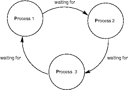
As an example, we will set up a deadlock with two processes. Suppose they share a duplex pipe and attempt to communicate with each other as follows:

def deadlock(in_pipe, out_pipe):
    item = in_pipe.recv()
    print('got an item:', item)
    out_pipe.send(item + 1)

def create_deadlock():
    pipe = multiprocessing.Pipe()
    other = multiprocessing.Process(target=deadlock, args=(pipe[0], pipe[1]))
    other.start()
    deadlock(pipe[1], pipe[0])

create_deadlock()

Both processes attempt to receive data first. Recall that the recv method blocks until an item is available. Since neither process has sent anything, both will wait indefinitely for the other to send it data, resulting in deadlock.

Synchronization operations must be properly aligned to avoid deadlock. This may require sending over a pipe before receiving, acquiring multiple locks in the same order, and ensuring that all threads reach the right barrier at the right time.

4.8.9 Conclusion

As we have seen, parallelism presents new challenges in writing correct and efficient code. As the trend of increasing parallelism at the hardware level will continue for the foreseeable future, parallel computation will become more and more important in application programming. There is a very active body of research on making parallelism easier and less error-prone for programmers. Our discussion here serves only as a basic introduction to this crucial area of computer science.