Bayes Theorem and Naive Bayes
Outline
- Bayes theorem
- Naive Bayes
- Naive Bayes in machine learning
- Naive Bayes for continuous input attributes
- Advantages and disadvantages
- Applications
Bayes Theorem everywhere in our life
What the chance of getting wet on our way to the university?
Probability
Probability gives a numerical description of how likely an event is to occur:
Probability of event(outcome)A:P(A)
- P(rainy) = 0.3
- P(snowy) = 0.05
- P(a coin lands on its head) = 0.5
P(A) + P(^A)=1.0
- P(rainy) + P(notrainy)=1,so P(notrainy)=0.7
Random variables
A random variable is avariable to describe the outcome of a random experiment
Consider a discrete random variable Weather
- P(Weather = rainy) = 0.3
- P(Weather = snowy) = 0.05
- P(Weather = sunny) = 0.4
- P(Weather = cloudy) = 0.25
Sum of the probabilities of all the outcomes is 1
Probability of multiple random variables
We may want to know the probability of two or more events occurring, e.g.,
- P(Weather = rainy, Season = winter) = 0.1
- P(Weather = rainy, Season = spring) = 0.15
- P(Weather = snowy, Season = summer) = 0
Joint probability of events A and B: P(A,B) or P(A B)
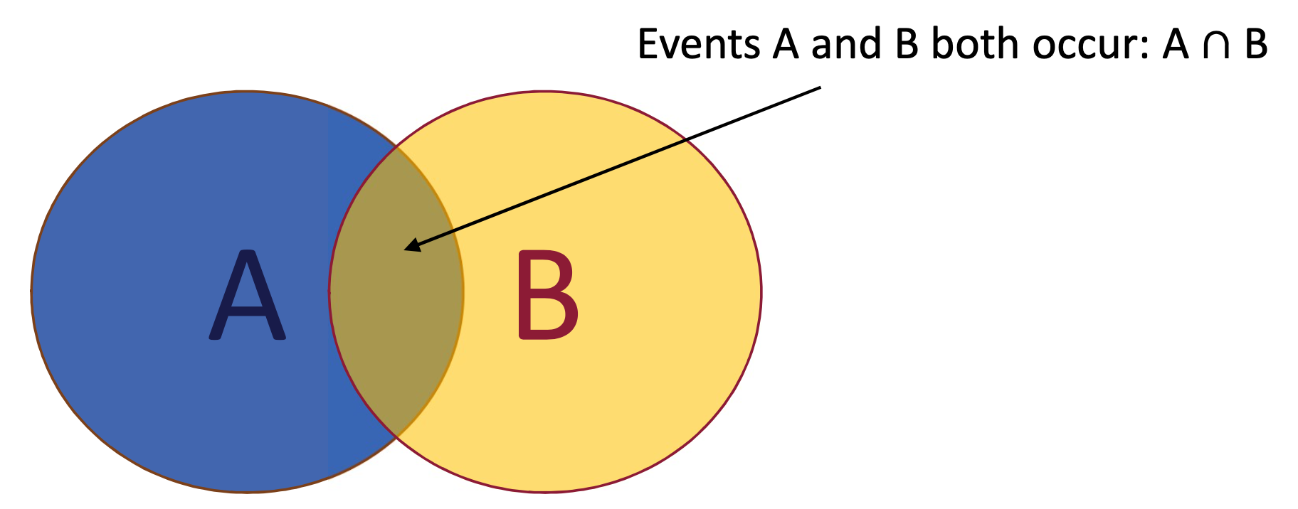
Conditional Probability
We may also be interested in the probability of an event given the occurrence of another event: P(A given B) or P(A $\mid$ B)
- P(Weather = rainy $\mid$ Season = winter) = 0.2
- P(Weather = rainy $\mid$ Season = spring) = 0.3
- P(Weather = snowy $\mid$ Season = winter) = 0.5
Calculating a conditional probability without the joint probability
Where:
- $A$: Hypothesis
- $B$: Evidence
- $P(A \mid B)$: Posterior Probability
- $P(A)$: Prior Probability
- $P(B \mid A$: Likelihood
- $P(B)$: Evidence Probability
Example
What the chance of getting wet on our way to the university?
- Probability of raining at Birmingham in March is 0.4
- Probability of taking an umbrella when raining is 0.9
- Probability of taking an umbrella when not raining is 0.2
Question
$P(raining \mid \hat {umbrella}) = ?$
Analyse
- $H = raining,\: E = \hat{umbrella}$
- $P(raining) = 0.4, \: P(\hat {raining} = 0.6)$
- $P(umbrella \mid raining) = 0.9, \: P(\hat{umbrella}\mid raining) = 0.1$
- $P(umbrella\mid \hat{raining}) = 0.2, \: P(\hat{umbrella} \mid \hat{raining}) = 0.8$
$\therefore \: $
Bayes Theorem
Example 2: Drug Testing
Suppose that a drug test will produce 99% true positive results for drug users and 99% true negative results for non-drug users. Suppose that 0.5% of people are users of the drug. What is the probability that a randomly selected individual with a positive test is a drug user? What is the probability that a randomly selected individual with a negative test is a drug user?
- Drug user: $drug$
- Non-drug user: $\hat{drug}$
- Positive: $+$
- Negative: $-$
Question
- $P(drug\mid +) = ?$
- $P(drug\mid -) = ?$
Analyse
$P(drug\mid +) = ?$
$P(drug\mid +) = P(drug) \cdot P(+\mid drug) \:/\: P(+)$
$P(+) = P(drug) \cdot P(+\mid drug) + P(\hat{drug}) \cdot P(+ \mid \hat{drug})=1.49\%$
$P(drug\mid +) = 0.5\% \times 99\% \:/\: 1.49\% \approx 33.2\%$
$P(drug\mid -) = ?$
$P(drug\mid -) = P(drug) \cdot P(-\mid drug) \:/\: P(-)$
$P(-) = P(drug) \cdot P(-\mid drug) + P(\hat{drug}) \cdot P(- \mid \hat{drug}) = 98.51\%$
$P(drug\mid -) = 0.5\% \times 1\% \:/\: 98.51\% \approx 0.005\%$
Revisit Drug Testing - Extension
Suppose that a drug test will produce 99% true positive results for drug users and 99% true negative results for non‐drug users. Suppose that 0.5% of people are users of the drug. What is the probability that a randomly selected individual with two positive tests is a drug user?
(assume that these two tests are mutually independent given whether if the person is a drug user or not)
Question
$P(drug\mid ++) = ?$
Analyse
$P(drug\mid ++) = P(drug) \cdot P(++\mid drug) \:/\: P(++)$
$P(++\mid drug) = P(+\mid drug) \cdot P(+\mid drug) = 99\% \cdot 99\% = 98.01\%$
$P(++) = P(drug)\cdot P(++\mid drug) + P(\hat{drug})\cdot P(++\mid \hat{drug}) = 0.5\%$
$P(drug\mid ++) = 98.01\%$
Interpretation of Bayes Theorem
- Probability measures a “degree of belief”
- Bayes theorem links the degree of belief in a hypothesis (proposition) before and after accounting for evidence
- $P(H \mid E) = P(H) \cdot P(E \mid H)\:/\:P(E)$, hypothesis $H$ and evidence $E$
- $P(H)$ is the initial degree of belief in $H$ (i.e. prior probability)
- $P(H\mid E)$ is the degree of belief having accounted for $E$
- Bayes theorem is not to determine our belief, but to update our belief
Bayes Theorem for Classification
- A machine learning model is to predict the relationships in the data, such as the relationship between features (i.e. attributes) (e.g. round, juicy, orange skin) and classes (e.g. orange, apple)
- Bayes theorem provides a probabilistic way to model the relationship in data: evidence = feature (input), hypothesis = class (output)
- It calculates the probability of an object given a number of
features (input $f_1,f_2,…, f_n$) belonging to a particular class (output $c$): $P(Y=c \mid X_1 = f_1, X_2 = f_2,…, X_n = f_n)$
Example: Tooth cavity testing
- To predict whether people have cavity when they do not do mouth wash by Bayes theorem
- Difference from the previous examples: unknown prior probability, likelihood, etc; need to learn from training examples
Analyse
- Input variable: Wash
- Output variable: Cavity
Training Set
| Person | Wash | Cavity |
|---|---|---|
| P1 | no | yes |
| P2 | no | yes |
| P3 | yes | yes |
| P4 | yes | no |
| P5 | yes | no |
| P6 | no | no |
Frequency Table
| Cavity = no | Cavity = yes | Total | |
|---|---|---|---|
| Wash = no | 1 | 2 | 3 |
| Wash = yes | 2 | 1 | 3 |
| Total | 3 | 3 | 6 |
Probabilities based on frequency table
$P(\hat{wash} \mid vacity) = \cfrac{2}{3}$
$P(wash \mid vacity) = \cfrac{1}{3}$
$P(cavity) = \cfrac{3}{6}$
$P(\hat{cavity}) = \cfrac{3}{6}$
$P(wash) = \cfrac{3}{6}$
$P(\hat{wash}) = \cfrac{3}{6}$
Now we can predict whether people have cavity when not doing mouth wash.
$P(cavity \mid \hat{wash})
= P(cavity) \cdot P(\hat{wash}\mid cavity) \:/\: P(\hat{wash})
\approx 67\%$$P(\hat{cavity} \mid \hat{wash}) \approx 33\%$
Bayes Theorem for multiple input attributes
To predict whether people have cavity when they do not do
mouth wash and have pain: $P(Y=cavity\mid X1=\hat{wash}, X2=pain)$
- Input variables: Wash, Pain
- Output variable: Cavity
Frequency table of joint input attributes
Training Set
| Person | Wash | Pain | Cavity |
|---|---|---|---|
| P1 | no | yes | yes |
| P2 | no | yes | yes |
| P3 | yes | yes | yes |
| P4 | yes | no | no |
| P5 | yes | no | no |
| P6 | no | no | no |
Frequency Table
| Cavity = no | Cavity = yes | Total | |
|---|---|---|---|
| Wash = no, Pain = no | 1 | 0 | 1 |
| Wash = no, Pain = yes | 0 | 2 | 2 |
| Wash = yes, Pain = no | 2 | 0 | 2 |
| Wash = yes, Pain = yes | 0 | 1 | 1 |
| Total | 3 | 3 | 6 |
- Downside: Number of possible combinations of input attributes can become very large
Naive Bayes
Naive Bayes = Bayes Theorem + Independence Assumption
Bayes Theorem:
Independence Assumption: Input attributes $f_1, …, f_n$ are mutually independent, conditional on any output, that is
- Naive Bayes
If there are m possible classes: $c_1, c_2, …, c_m$, based on the independent assumption we have
As $P(f_1, …, f_n)$ is the same (i.e. a constant) for any class $c$, we can denote $P(f_1, …, f_n) = \cfrac{1}{\alpha}$,
where $\alpha$ is a normalised factor
Therefore
Frequency table of joint input attributes
Training Set
| Person | Wash | Pain | Cavity |
|---|---|---|---|
| P1 | no | yes | yes |
| P2 | no | yes | yes |
| P3 | yes | yes | yes |
| P4 | yes | no | no |
| P5 | yes | no | no |
| P6 | no | no | no |
Frequency Table
| Cavity = no | Cavity = yes | Total | |
|---|---|---|---|
| Wash = no, Pain = no | 1 | 0 | 1 |
| Wash = no, Pain = yes | 0 | 2 | 2 |
| Wash = yes, Pain = no | 2 | 0 | 2 |
| Wash = yes, Pain = yes | 0 | 1 | 1 |
| Total | 3 | 3 | 6 |
Therefore
Frequency Table
| Cavity = no | Cavity = yes | Total | |
|---|---|---|---|
| Wash = no | 1 | 2 | 3 |
| Wash = yes | 2 | 1 | 3 |
| Total | 3 | 3 | 6 |
| Cavity = no | Cavity = yes | Total | |
|---|---|---|---|
| Pain = no | 3 | 0 | 3 |
| Pain = yes | 0 | 3 | 3 |
| Total | 3 | 3 | 6 |
Naive Bayes classifier
and
Where
Categorical naive Bayes
Categorical naive Bayes: all the input attributes are categorical variables.
- A categorical variable is a variable that can take on one of a limited number of possible values
- This contrasts with numerical (continuous) naive Bayes, where
some input variable can be represented by real numbers (i.e. infinite possible attribute values)
Categorical vs Numerical attributes
Training Set
| Person | Wash | Pain | Cavity |
|---|---|---|---|
| P1 | no | yes | yes |
| P2 | no | yes | yes |
| P3 | yes | yes | yes |
| P4 | yes | no | no |
| P5 | yes | no | no |
| P6 | no | no | no |
Categorical
| Person | Wash | Cavity |
|---|---|---|
| P1 | no | yes |
| P2 | no | yes |
| P3 | yes | yes |
| P4 | yes | no |
| P5 | yes | no |
| P6 | no | no |
Numerical
| Person | Sugar (grams) | Cavity |
|---|---|---|
| P1 | 40 | yes |
| P2 | 35 | yes |
| P3 | 60 | yes |
| P4 | 20 | no |
| P5 | 30 | no |
| P6 | 17 | no |
Deal with numerical input attributes by discretising values
Transform numerical input values into categories (i.e., discrete values)
E.g.: Sugar $\rightarrow$ small, medium, large
However, a person may consider large as >30g. Another may consider it as >25g
If the amount of sugar is large when $\ge$ 30g, should 29.9g be considered medium? Not large?
This level of subjectiveness and crispiness may lead to loss of information
Probability Function
Probability Function describes the probability distribution of a random variable, i.e., the probabilities of occurrence of different possible outcomes in an experiment.
Probability Mass Function: the random variable is discrete
| Person | Wash | Cavity |
|---|---|---|
| P1 | no | yes |
| P2 | no | yes |
| P3 | yes | yes |
| P4 | yes | no |
| P5 | yes | no |
| P6 | no | no |
Probability Mass Function for P(Wash|cavity):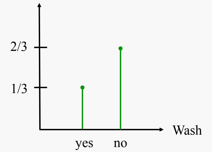
- X axis represents possible values of the feature
- Y axis represents the probability of the feature being a value given a particular class
Probability Density Function
Probability Density Function is a probability function where the variable is continuous.
| Person | Sugar (grams) | Cavity |
|---|---|---|
| P1 | 40 | yes |
| P2 | 35 | yes |
| P3 | 60 | yes |
| P4 | 20 | no |
| P5 | 30 | no |
| P6 | 17 | no |
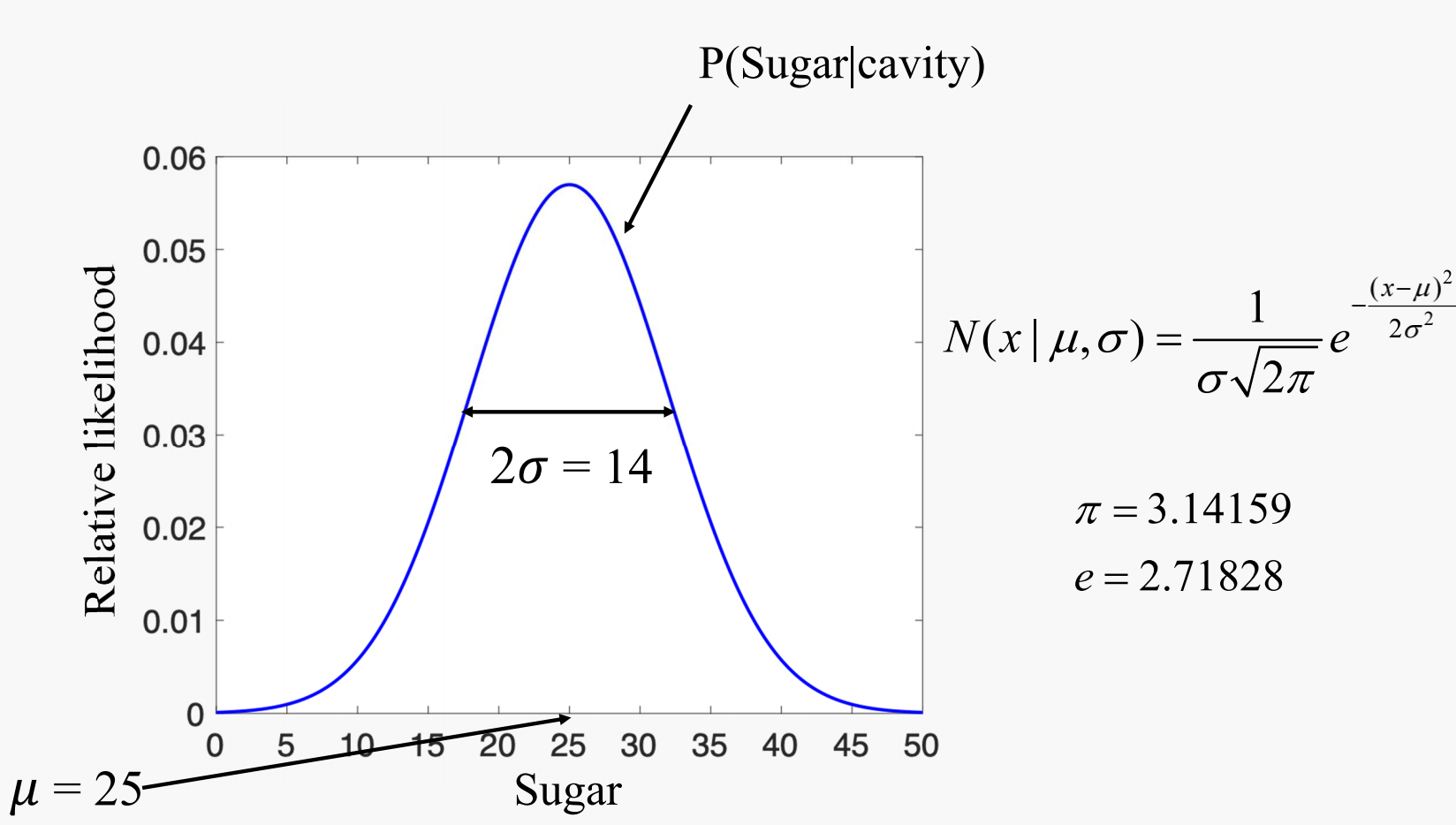
- Shape of the function: Assume the examples drawn from Gaussian Distribution (aka normal Distribution).
- Shape is controlled by two parameters: Mean ($\mu$) and Standard Deviation ($\sigma$), determined by the training examples.
Gaussian Distribution $N(x \mid \mu , \sigma )$: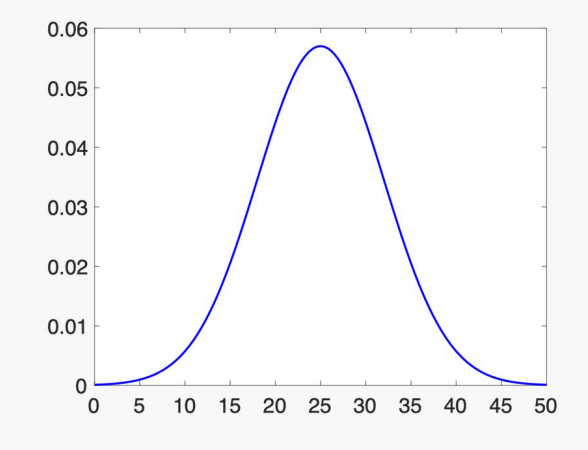
Gaussian Distribution
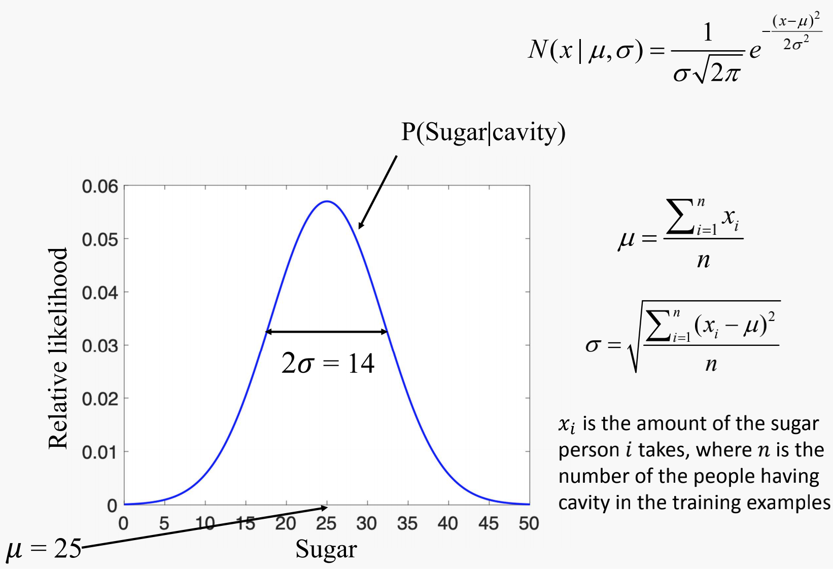
Probability Density Function calculation for people having cavity
$x_i$ is the amount of the sugar person takes, where is the number of the people having cavity in the training examples.
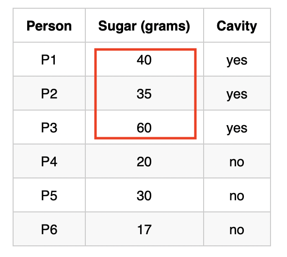
Therefore
Use $\mu$ and $\sigma$ to plot the Gaussian distribution graph:
Sugar is $x$ and $P(Sugar\mid cavity)$ is $N(x \mid \mu, \sigma)$.
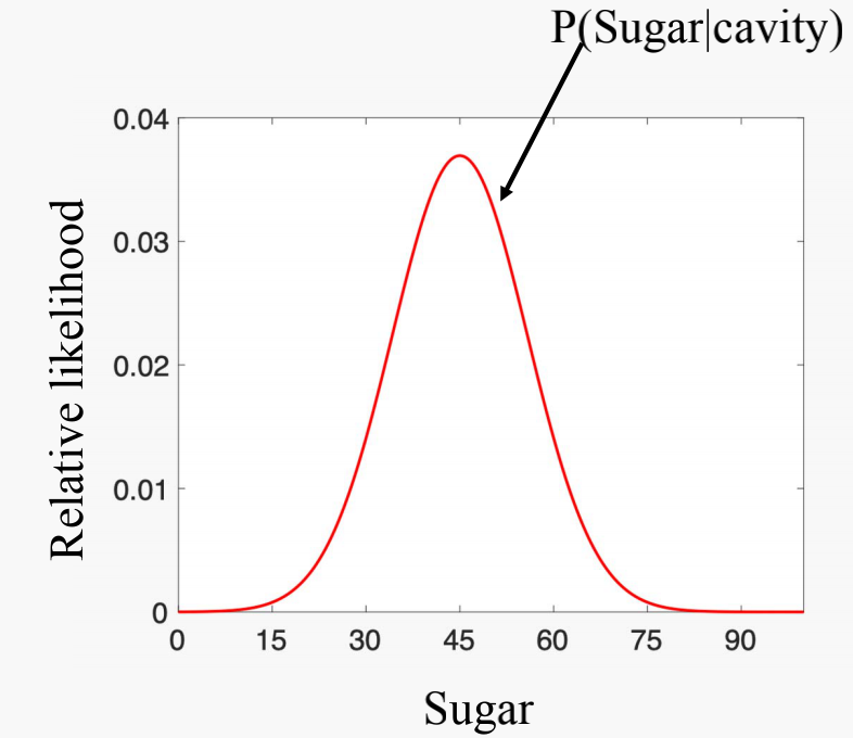
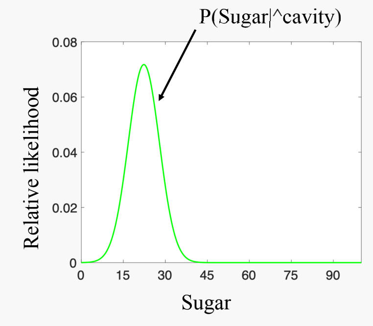
Probability Density Function calculation for people not having cavity
$x_i$ is the amount of the sugar person takes, where is the number of the people not having cavity in the training examples.
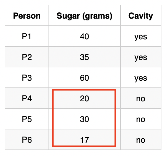
Therefore
Use $\mu$ and $\sigma$ to plot the Gaussian distribution graph:
Sugar is $x$ and $P(Sugar\mid \hat{cavity})$ is $N(x \mid \mu, \sigma)$.
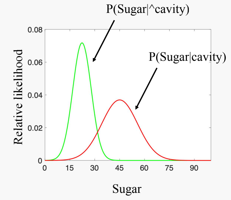
Probability distribution functions
Probability distribution function of Sugar given cavity or no cavity:
| Person | Sugar (grams) | Cavity |
|---|---|---|
| P1 | 40 | yes |
| P2 | 35 | yes |
| P3 | 60 | yes |
| P4 | 20 | no |
| P5 | 30 | no |
| P6 | 17 | no |
General idea
Decide on a type of probability density function (usually Gaussian distribution) for each numerical input attribute $X$.
Determine the parameters of the probability function for each possible output attribute value (i.e.$c_1, c_2, …, c_m$) according to the training examples.
Use the obtained probability function for $c_i$ to calculate $P(X =f \mid Y = c_i)$ for the corresponding input value $f$.
Example
We want to predict if a person has cavity when they do not do mouth wash and take sugar 20 grams everyday.
We need to calculate $P(cavity \mid \hat{wash}, Sugar=20)$ and $P(\hat{cavity}\mid \hat{wash}, Sugar=20)$.
| Person | Wash | Sugar (grams) | Cavity |
|---|---|---|---|
| P1 | no | 40 | yes |
| P2 | no | 35 | yes |
| P3 | yes | 60 | yes |
| P4 | yes | 20 | no |
| P5 | yes | 30 | no |
| P6 | no | 17 | no |
Calculate $P(Sugar=20 \mid cavity)$:
- Probability Density Function of the variable Sugar given cavity

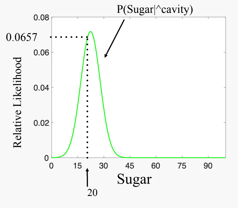
Calculate $P(Sugar=20 \mid \hat{cavity})$:
- Probability Density Function of the variable Sugar given no cavity
Result
Predict if people have cavity when they do not do mouth wash and take sugar 20 grams everyday.
$P(cavity \mid \hat{wash}, Sugar=20)
= \alpha \times \cfrac{3}{6} \times \cfrac{2}{3} \times0.0025 = 0.00083\alpha$
$P(\hat{cavity} \mid \hat{wash}, Sugar=20)
= \alpha \times \cfrac{3}{6} \times \cfrac{1}{3} \times0.0657 = 0.01095\alpha$
Predicted results: No cavity
Advantages and disadvantages of naive Bayes
Advantages:
- Does very well in classification, especially on high‐dimensional dataset
- Requires a small amount of training data; training is very quick
- Easy to build/implement
Disadvantages:
- Requires the assumption of independent input attributes
- For continuous input attributes, it assumes a certain probability distribution for input attributes
- Not work very well for regression
Applications
To categorise emails, e.g., spam or not spam
To check a piece of text expressing positive emotions, or negative emotions
To classify a news article about technology, politics, or sports
Software defect prediction
Medical diagnosis
…
Logic
Outline
- Propositional Logic
- First Order Logic
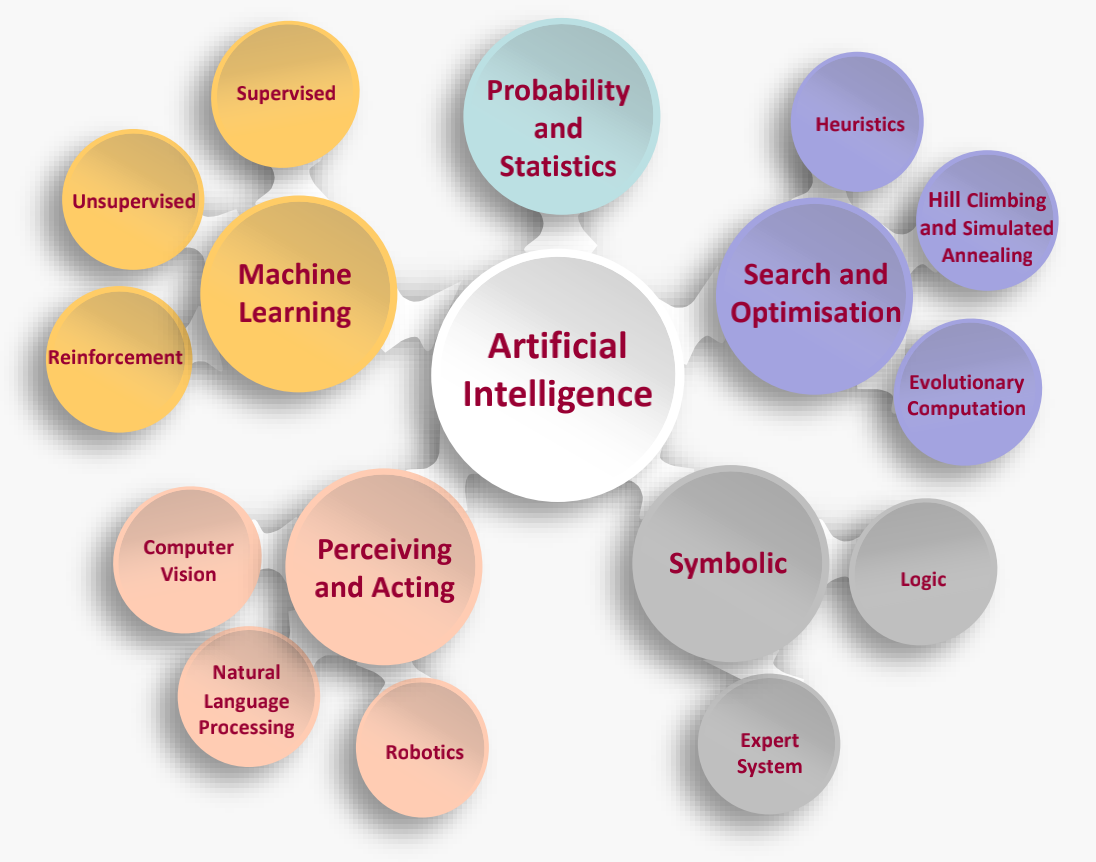
AI Branches
Propositional Logic
- A proposition is simply a statement, either true or false
- There is no concept of a degree of truth
- Propositional logic deals with logical relationships between propositions (statements, claims) taken as wholes
- Such letters are not variables, called propositional constant

P = “John is wearing a red coat”
Compound proposition
Compound proposition is constructed by individual propositions and connectives (logical operators)
P and Q (conjunction of two propositions, denoted by $\wedge$)
- John is wearing a red coat and he’s stolen a jeep
P or Q (disjunction of two propositions, denoted by $\vee$)
- John is at the library or he is studying
If P then Q (conditional of one proposition implying the
other, denoted by $\rightarrow$)- If John is at the library, then he is preparing the exam
Not P (contradictory of the proposition, denoted by $\neg$)
- It is not the case that John is at the library
Connectives
If (A or B) then (C and not D)
- $A \vee B \rightarrow C \wedge \neg D$
Given the truth value of A, B, C, D, is this compound proposition true or false?
Truth table
A truth table shows how the truth or falsity of a compound statement depends on the truth or falsity of the individual statements from which it’s constructed.
| P | Q | P $\wedge$ Q | P $\vee$ Q | P$\rightarrow$Q | $\neg$P |
|---|---|---|---|---|---|
| T | T | T | T | T | F |
| T | F | F | T | F | F |
| F | T | F | T | T | T |
| F | F | F | F | T | T |
Inclusive/exclusive OR
Inclusive or: A triangle can be defined as a polygon with three sides or a polygon with three vertices
Exclusive or (denoted xor): The coin landed either heads or tails
| P | Q | P $\vee$ Q | P$\bigoplus$Q |
|---|---|---|---|
| T | T | T | F |
| T | F | T | T |
| F | T | T | T |
| F | F | F | F |
Conditionals
Conditional can be thought of as an “if”statement
If I miss the bus, then I will be late for work
| P | Q | P $\rightarrow$ Q |
|---|---|---|
| T | T | T |
| T | F | F |
| F | T | T |
| F | F | T |
When a conditional is false?
If I study hard, then I will pass the test
P: I study hard; Q: I pass the test
- Case 1: P is true, Q is true
- I studied hard, I passed the test
- Case 2: P is true, Q is false
- I studied hard, I did not pass the test
- Case 3: P is false, Q is true
- I did not study hard, I passed the test
- Case 4: P is false, Q is false
- I did not study hard, I did not pass the test
| P | Q | P $\rightarrow$ Q |
|---|---|---|
| T | T | T |
| T | F | F |
| F | T | T |
| F | F | T |
Biconditionals
The bidirectional (denoted P $\leftrightarrow$ Q) implies in both directions
“(If P then Q) and (If Q then P)”
P iff Q (is read P if and only if Q)
(During the day) The sun is shining iff there are no clouds covering the sun
If I have a pet goat, then my homework will be eaten (true)
If my homework is eaten, then I have a pet goat (not true)
| P | Q | P $\leftrightarrow$ Q |
|---|---|---|
| T | T | T |
| T | F | F |
| F | T | F |
| F | F | T |
Contradictories
Contradictory of P (¬P or not P): a claim that always has the opposite truth value of P
P: “John is at the movies”
It can be read “it is not the case that John is at the movies”
Arguments
An argument is a set of propositions, called the premises, intended to determine the truth of another statement, called the conclusion
Multiple statements
Premises: Supporting statements
Conclusion: Statement that follows from premises
- $P \leftrightarrow Q$
- $\cfrac{Q}{\therefore P}$
P: The river is flooded; Q: It rained heavily
Validity
- An argument is valid if the premises lead to the conclusion presented
- P: I run Marathon, Q: I am exhausted
Soundness
A sound argument is valid and all of its premises are true
A unsound argument lacks validity or truth
Common arguments: Valid or not
$((P \rightarrow Q) \wedge Q) \therefore P$
- P implies Q and Q, therefore P
$((P \rightarrow Q) \wedge \neg Q) \therefore \neg P$
- P implies Q and not Q, therefore not P
$((P \rightarrow Q) \wedge (Q \rightarrow R)) \therefore P \rightarrow R$
- P implies Q and Q implies R, therefore P implies R
$(P \leftrightarrow Q) \therefore (P \wedge Q) \vee (\neg P \wedge \neg Q)$
- P iff Q, therefore (P and Q) or (not P and not Q)
Argument $((P \rightarrow Q) \wedge Q) \therefore P$
| P | Q | $P \rightarrow Q$ | $(P \rightarrow Q) \wedge Q$ | $((P \rightarrow Q) \wedge Q) \rightarrow P$ |
|---|---|---|---|---|
| T | T | T | T | T |
| T | F | F | F | T |
| F | T | T | T | F |
| F | F | T | F | T |
Not valid
Argument $((P \rightarrow Q) \wedge \neg Q) \therefore \neg P$
| P | Q | $P \rightarrow Q$ | $\neg Q$ | $(P \rightarrow Q) \wedge \neg Q$ | $\neg P$ | $((P \rightarrow Q) \wedge \neg Q) \rightarrow \neg P$ |
|---|---|---|---|---|---|---|
| T | T | T | F | F | F | T |
| T | F | F | T | F | F | T |
| F | T | T | F | F | T | T |
| F | F | T | T | T | T | T |
Valid
First Order Logic
First-order logic (aka predicate logic) is a generalisation of propositional logic
First-order logic is a powerful language that uses quantified variables over objects and allows the use of sentences that contain variables
First-order logic adds predicates and quantifiers to propositional logic
Predicates
“Socrates is a philosopher”
“Plato is a philosopher”
The predicate “is a philosopher” occurs in both sentences, which have a common structure “𝑥 is a philosopher”, “𝑥” can be Socrates or Plato
Such a sentence can be represented as Predicate(term1, term2, …); for example, philosopher(𝑥), philosopher(Socrates)
First-order logic uses Predicate(term1, term2…) to represent basic sentences, where terms can be variables/constants
—
Birds fly:
- fly(birds)
John respects his parents:
- respect(John, parents)
x is greater than y:
- greater(x, y)
1 is greater than 2:
- greater(1, 2)
Connectives
We can use logic connectives on predicates
$philosopher(x) \rightarrow scholar(x)$
- “x is a philosopher” implies that “x is a scholar”
$respect(John, parents) \wedge respect(John, wife)$
- “John respects his parents” and “John respects his wife”
Quantifiers
A quantifier turns a sentence about something having some property into a sentence about the number (quantity) of things having the property
Universal quantifier is “for all” (i.e. “for every”)
- $\forall x \:\: P(x)$: “For all x, x is P”.
- $\forall x \:\: philosopher(x)$: “For all x, x is philosopher”.
Existential quantifier is “for some” (i.e. “there exists”)
- $\exists x \:\: P(x)$: “For some x, x is P”.
- $\exists x \:\: philosopher(x)$: “For some x, x is philosopher”.
Universal quantifier
- All man drink coffee
- $\forall x \:\: man(x) \rightarrow drink(x, coffee)$
- In universal quantifier we use implication “$\rightarrow$”
Existential quantifier
- Some boys are intelligent
- $\exists x\:\: boys(x) \wedge intelligent(x)$
- In existential quantifier we use and “$\wedge$”
Examples
All philosophers are scholars
- For all x, where “x is a philosopher” then “x is a scholar”
- $\forall x\:\: philosopher(x) \rightarrow scholar(x)$
Every man respects his parents
- $\forall x\:\: man(x) \rightarrow respect(x, parents)$
Some boys play football
- $\exists x\:\: boy(x) \wedge play(x, football)$
Not all students like both mathematics and science
- $\neg \forall x\:\: [student(x) \rightarrow like(x, mathematics) ∧ like(x, science)]$